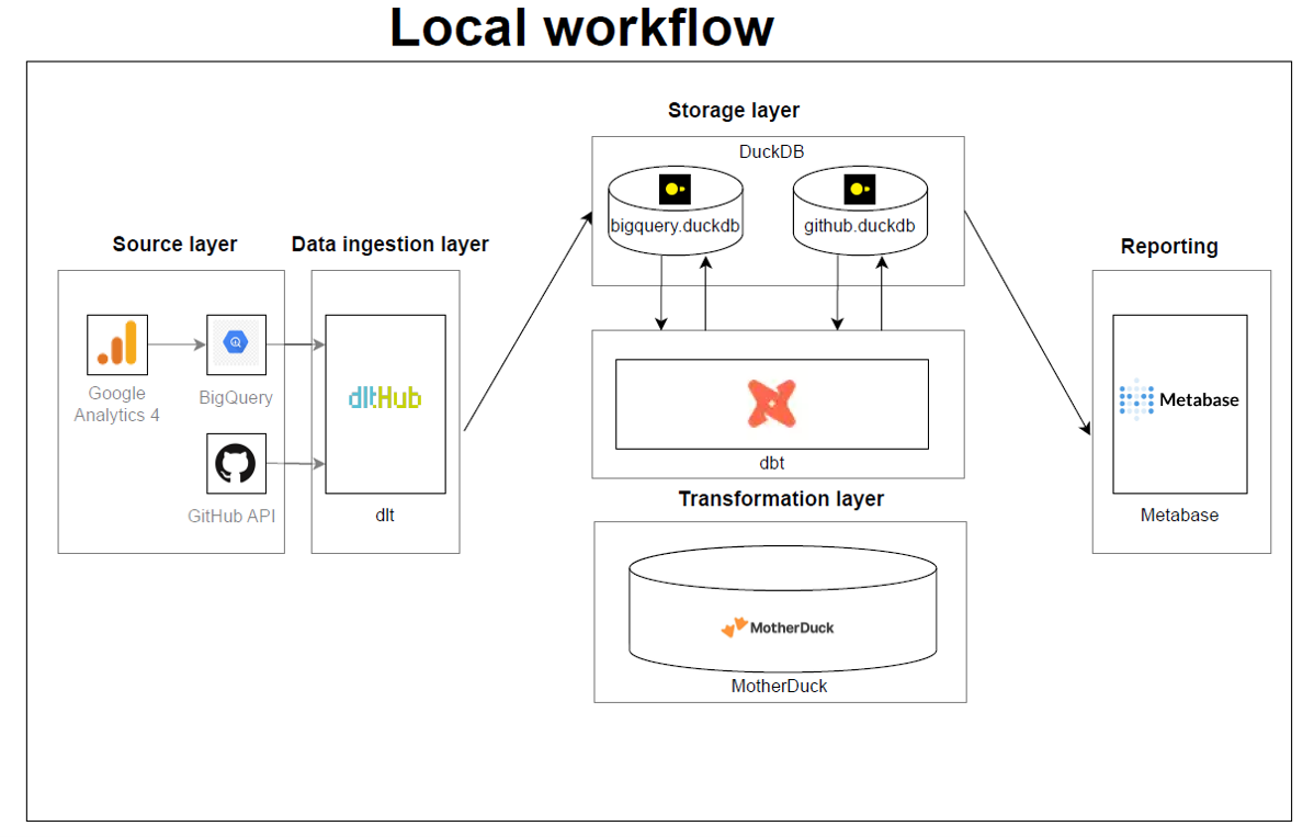
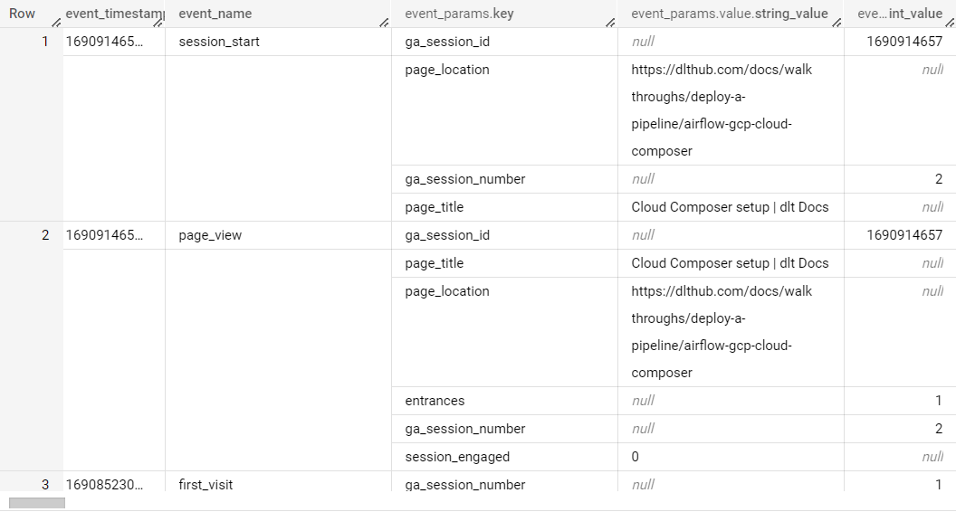
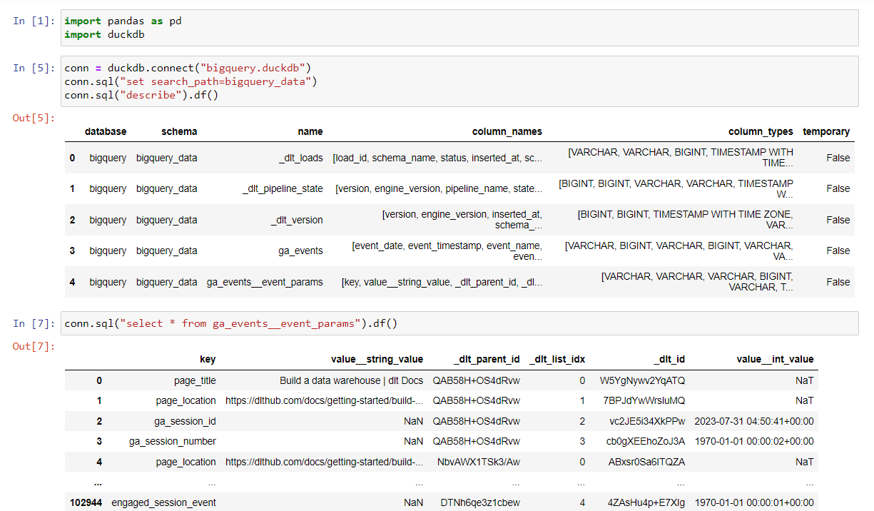
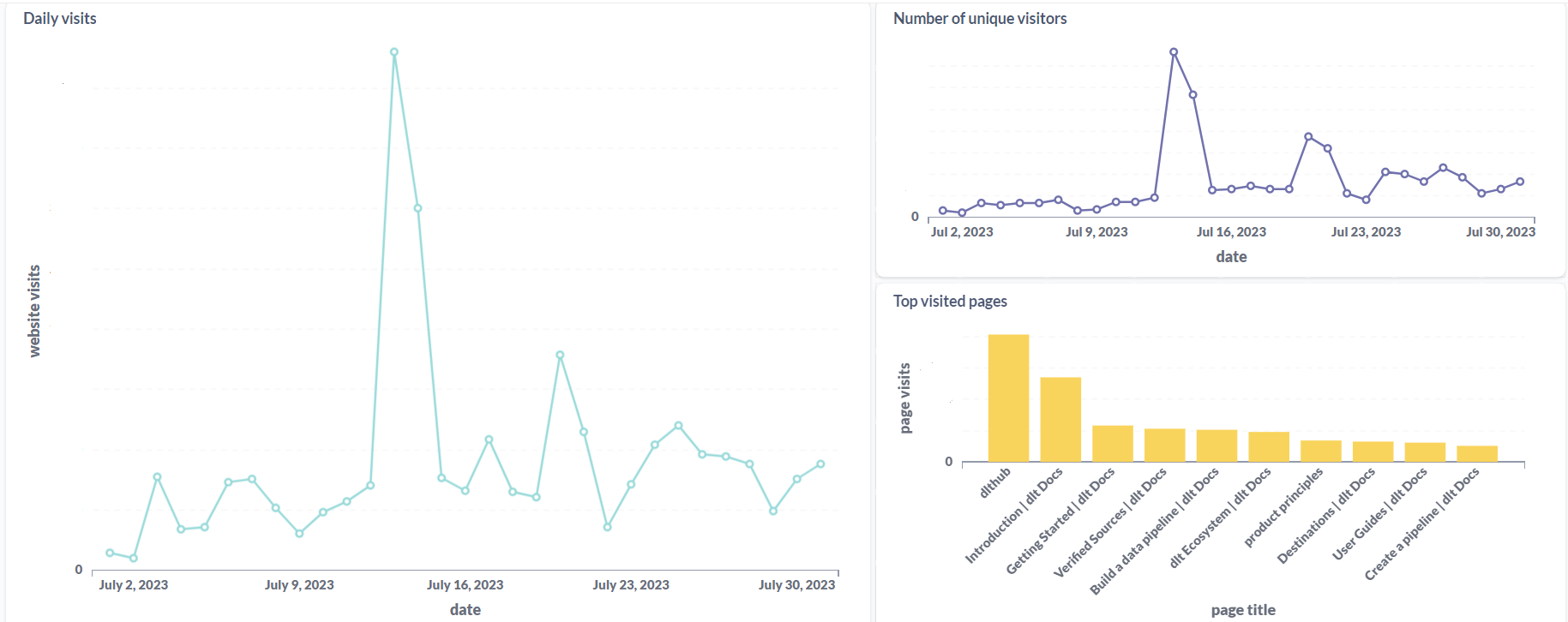
15 posts tagged with "dlt"

View All Tags

· 12 min read
Anuun Chinbat

It's been nearly half a century since cron was first introduced, and now we have a handful orchestration tools that go way beyond just scheduling tasks. With data folks constantly debating about which tools are top-notch and which ones should leave the scene, it's like we're at a turning point in the evolution of these tools. By that I mean the term 'orchestrator' has become kind of a catch-all, and that's causing some confusion because we're using this one word to talk about a bunch of different things.

dates

Think about the word “date.” It can mean a fruit, a romantic outing, or a day on the calendar, right? We usually figure out which one it is from the context, but what does context mean when it comes to orchestration? It might sound like a simple question, but it's pretty important to get this straight.

And here's a funny thing: some people, after eating an odd-tasting date (the fruit, of course), are so put off that they naively swear off going on romantic dates altogether. It's an overly exaggerated figurative way of looking at it, but it shows how one bad experience can color our view of something completely different. That's kind of what's happening with orchestration tools. If someone had a bad time with one tool, they might be overly critical towards another, even though it might be a totally different experience.

So the context in terms of orchestration tools seems to be primarily defined by one thing - WHEN a specific tool was first introduced to the market (aside from the obvious factors like the technical background of the person discussing these tools and their tendency to be a chronic complainer 🙄).


IT'S ALL ABOUT TIMING!
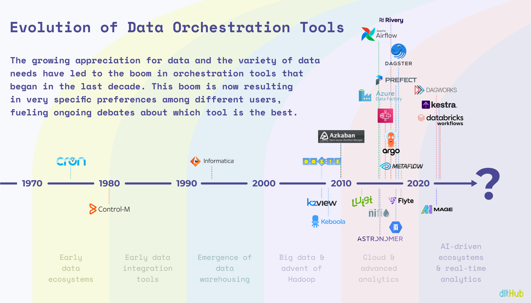
evolution-of-data-orchestration

The Illegitimate Child

Cron was initially released in 1975 and is undoubtedly the father of all scheduling tools, including orchestrators, but I’m assuming Cron didn’t anticipate this many offspring in the field of data (or perhaps it did). As Oracle brought the first commercial relational database to market in 1979, people started to realize that data needs to be moved on schedule, and without manual effort. And it was doable, with the help of Control-M, though it was more of a general workflow automation tool that didn’t pay special attention to data workflows.

Basically, since the solutions weren’t data driven at that time, it was more “The job gets done, but without a guarantee of data quality.”

Finally Adopted

Unlike Control-M, Informatica was designed for data operations in mind from the beginning. As data started to spread across entire companies, advanced OLAPs started to emerge with a broad use of datawarehousing. Now data not only needed to be moved, but integrated across many systems and users. The data orchestration solution from Informatica was inevitably influenced by the rising popularity of the contemporary drag-and-drop concept, that is, to the detriment of many modern data engineers who would recommend to skip Informatica and other GUI based ETL tools that offer ‘visual programming’.

As the creator of Airflow, Max Beauchemin, said: “There's a multitude of reasons why complex pieces of software are not developed using drag and drop tools: it's that ultimately code is the best abstraction there is for software.

To Be Free, That Is, Diverse

With traditional ETL tools, such as IBM DataStage and Talend, becoming well-established in the 1990s and early 2000s, the big data movement started gaining its momentum with Hadoop as the main star. Oozie, later made open-source in 2011, was tasked with workflow scheduling of Hadoop jobs, with closed-source solutions, like K2View starting to operate behind the curtains.

Fast forward a bit, and the scene exploded, with Airflow quickly becoming the heavyweight champ, while every big data service out there began rolling out their own orchestrators. This burst brought diversity, but with diversity came a maze of complexity. All of a sudden, there’s an orchestrator for everyone — whether you’re chasing features or just trying to make your budget work 👀 — picking the perfect one for your needs has gotten even trickier.
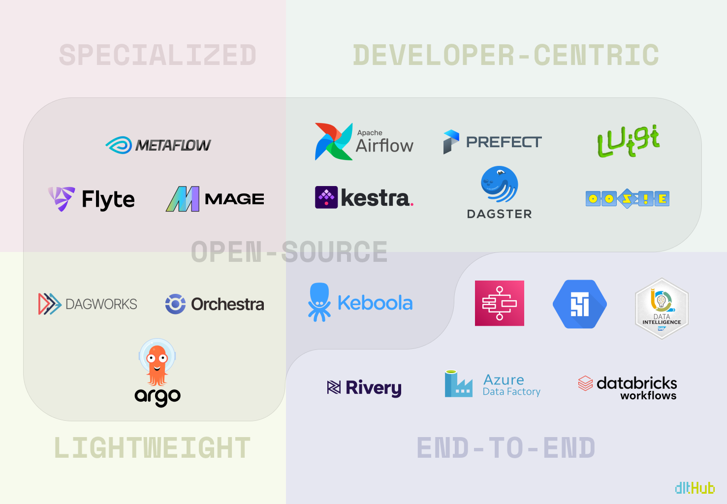
types

The Bottom Line

The thing is that every tool out there has some inconvenient truths, and real question isn't about escaping the headache — it's about choosing your type of headache. Hence, the endless sea of “versus” articles, blog posts, and guides trying to help you pick your personal battle.

A Redditor: “Everyone has hated all orchestration tools for all time. People just hated Airflow less and it took off.“

What I'm getting at is this: we're all a bit biased by the "law of the instrument." You know, the whole “If all you have is a hammer, everything looks like a nail” thing. Most engineers probably grabbed the latest or most hyped tool when they first dipped their toes into data orchestration and have stuck with it ever since. Sure, Airflow is the belle of the ball for the community, but there's a whole lineup of contenders vying for the spotlight.

law-of-instrument

And there are obviously those who would relate to the following:

reddit-screenshot


A HANDY DETOUR POUR TOI 💐

The Fundamentals

About Airflow

Miscellaneous


WHAT THE FUTURE HOLDS...

I'm no oracle or tech guru, but it's pretty obvious that at their core, most data orchestration tools are pretty similar. They're like building blocks that can be put together in different ways—some features come, some go, and users are always learning something new or dropping something old. So, what's really going to make a difference down the line is NOT just about having the coolest features. It's more about having a strong community that's all in on making the product better, a welcoming onboarding process that doesn't feel like rocket science, and finding that sweet spot between making things simple to use and letting users tweak things just the way they like.

In other words, it's not just about what the tools can do, but how people feel about using them, learning them, contributing to them, and obviously how much they spend to maintain them. That's likely where the future winners in the data orchestration game will stand out. But don’t get me wrong, features are important — it's just that there are other things equally important.


I’ve been working on this article for a WHILE now, and, honestly, it's been a bit of a headache trying to gather any solid, objective info on which data orchestration tool tops the charts. The more I think about it, the more I realise it's probably because trying to measure "the best" or "most popular" is a bit like trying to catch smoke with your bare hands — pretty subjective by nature. Plus, only testing them with non-production level data probably wasn't my brightest move.

However, I did create a fun little project where I analysed the sentiment of comments on articles about selected data orchestrators on Hacker News and gathered Google Trends data for the past year.

Just a heads-up, though: the results are BY NO MEANS reliable and are skewed due to some fun with words. For instance, searching for “Prefect” kept leading me to articles about Japanese prefectures, “Keboola” resulted in Kool-Aid content, and “Luigi”... well, let’s just say I ran into Mario’s brother more than once 😂.


THE FUN LITTLE PROJECT

Straight to the GitHub repo.

I used Dagster and dlt to load data into Snowflake, and since both of them have integrations with Snowflake, it was easy to set things up and have them all running:
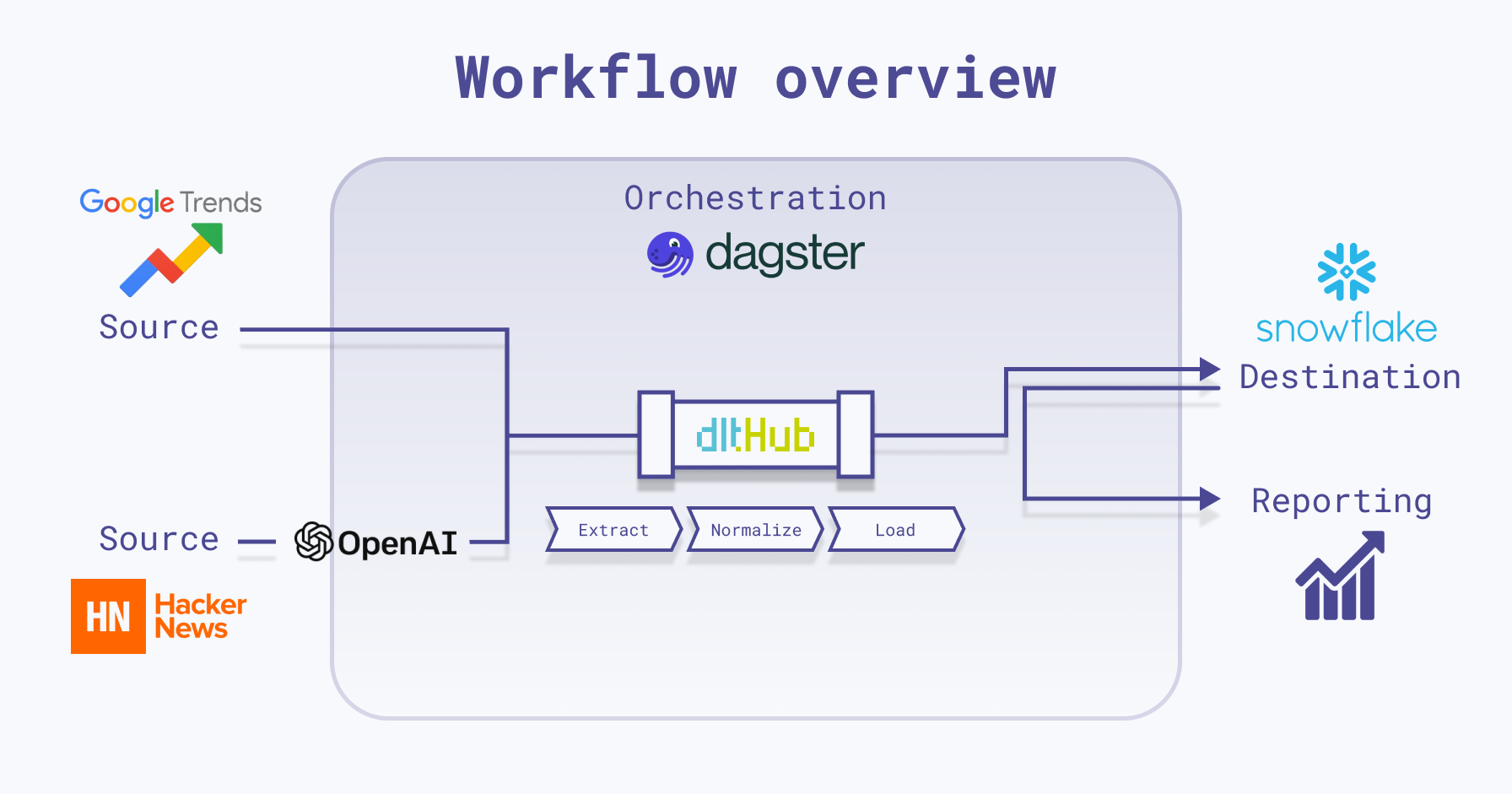
Pipeline overview

This project is very minimal, including just what's needed to run Dagster locally with dlt. Here's a quick breakdown of the repo’s structure:

  1. .dlt: Utilized by the dlt library for storing configuration and sensitive information. The Dagster project is set up to fetch secret values from this directory as well.
  2. charts: Used to store chart images generated by assets.
  3. dlt_dagster_snowflake_demo: Your Dagster package, comprising Dagster assets, dlt resources, Dagster resources, and general project configurations.

Dagster Resources Explained

In the resources folder, the following two Dagster resources are defined as classes:

  1. DltPipeline: This is our dlt object defined as a Dagster ConfigurableResource that creates and runs a dlt pipeline with the specified data and table name. It will later be used in our Dagster assets to load data into Snowflake.

    class DltPipeline(ConfigurableResource):
    # Initialize resource with pipeline details
    pipeline_name: str
    dataset_name: str
    destination: str

    def create_pipeline(self, resource_data, table_name):
    """
    Creates and runs a dlt pipeline with specified data and table name.

    Args:
    resource_data: The data to be processed by the pipeline.
    table_name: The name of the table where data will be loaded.

    Returns:
    The result of the pipeline execution.
    """

    # Configure the dlt pipeline with your destination details
    pipeline = dlt.pipeline(
    pipeline_name=self.pipeline_name,
    destination=self.destination,
    dataset_name=self.dataset_name
    )

    # Run the pipeline with your parameters
    load_info = pipeline.run(resource_data, table_name=table_name)
    return load_info
  2. LocalFileStorage: Manages the local file storage, ensuring the storage directory exists and allowing data to be written to files within it. It will be later used in our Dagster assets to save images into the charts folder.

dlt Explained

In the dlt folder within dlt_dagster_snowflake_demo, necessary dlt resources and sources are defined. Below is a visual representation illustrating the functionality of dlt:
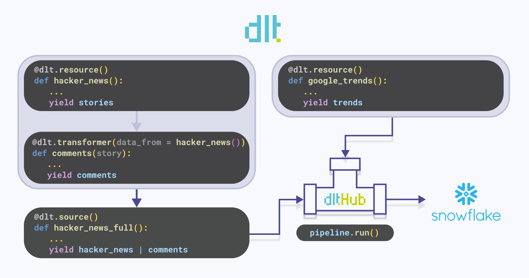
dlt explained

  1. hacker_news: A dlt resource that yields stories related to specified orchestration tools from Hackernews. For each tool, it retrieves the top 5 stories that have at least one comment. The stories are then appended to the existing data.

    Note that the write_disposition can also be set to merge or replace:

    • The merge write disposition merges the new data from the resource with the existing data at the destination. It requires a primary_key to be specified for the resource. More details can be found here.
    • The replace write disposition replaces the data in the destination with the data from the resource. It deletes all the classes and objects and recreates the schema before loading the data.

    More details can be found here.

  2. comments: A dlt transformer - a resource that receives data from another resource. It fetches comments for each story yielded by the hacker_news function.

  3. hacker_news_full: A dlt source that extracts data from the source location using one or more resource components, such as hacker_news and comments. To illustrate, if the source is a database, a resource corresponds to a table within that database.

  4. google_trends: A dlt resource that fetches Google Trends data for specified orchestration tools. It attempts to retrieve the data multiple times in case of failures or empty responses. The retrieved data is then appended to the existing data.

As you may have noticed, the dlt library is designed to handle the unnesting of data internally. When you retrieve data from APIs like Hacker News or Google Trends, dlt automatically unpacks the nested structures into relational tables, creating and linking child and parent tables. This is achieved through unique identifiers (_dlt_id and _dlt_parent_id) that link child tables to specific rows in the parent table. However, it's important to note that you have control over how this unnesting is done.

The Results

Alright, so once you've got your Dagster assets all materialized and data loaded into Snowflake, let's take a peek at what you might see:
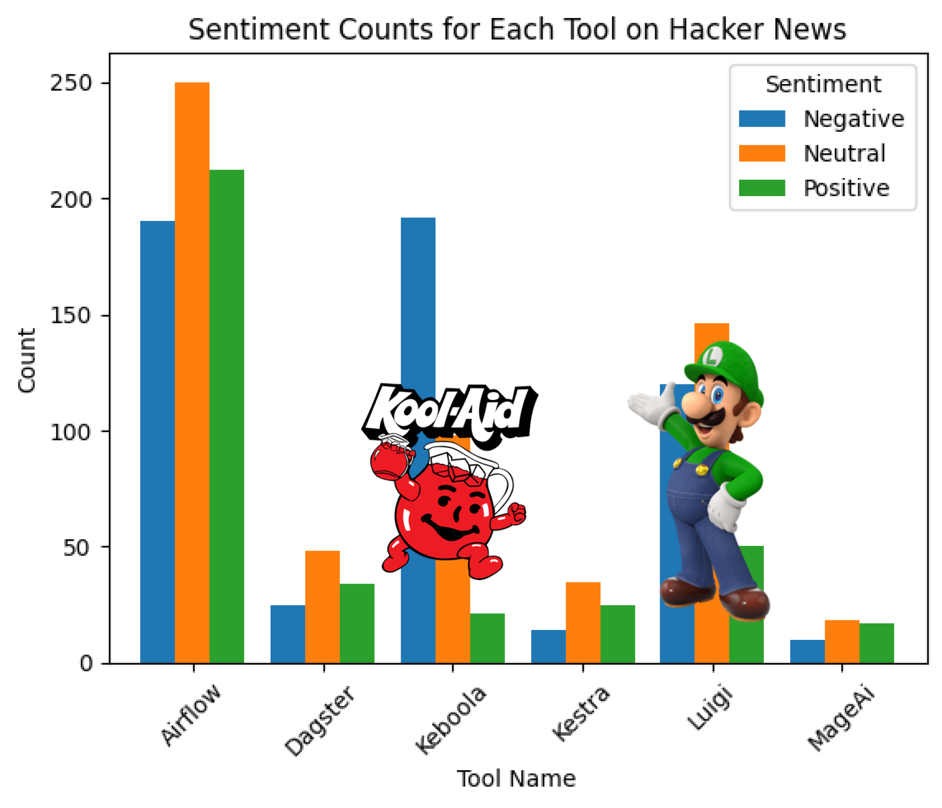
sentiment counts

I understand if you're scratching your head at first glance, but let me clear things up. Remember those sneaky issues I mentioned with Keboola and Luigi earlier? Well, I've masked their charts with the respective “culprits”.

Now, onto the bars. Each trio of bars illustrates the count of negative, neutral, and positive comments on articles sourced from Hacker News that have at least one comment and were returned when searched for a specific orchestration tool, categorized accordingly by the specific data orchestration tool.

What's the big reveal? It seems like Hacker News readers tend to spread more positivity than negativity, though neutral comments hold their ground.

And, as is often the case with utilizing LLMs, this data should be taken with a grain of salt. It's more of a whimsical exploration than a rigorous analysis. However, if you take a peek behind Kool Aid and Luigi, it's intriguing to note that articles related to them seem to attract a disproportionate amount of negativity. 😂


IF YOU'RE STILL HERE

… and you're just dipping your toes into the world of data orchestration, don’t sweat it. It's totally normal if it doesn't immediately click for you. For beginners, it can be tricky to grasp because in small projects, there isn't always that immediate need for things to happen "automatically" - you build your pipeline, run it once, and then bask in the satisfaction of your results - just like I did in my project. However, if you start playing around with one of these tools now, it could make it much easier to work with them later on. So, don't hesitate to dive in and experiment!

… And hey, if you're a seasoned pro about to drop some knowledge bombs, feel free to go for it - because what doesn’t challenge us, doesn’t change us 🥹. (*Cries in Gen Z*)

· 5 min read
Matthaus Krzykowski

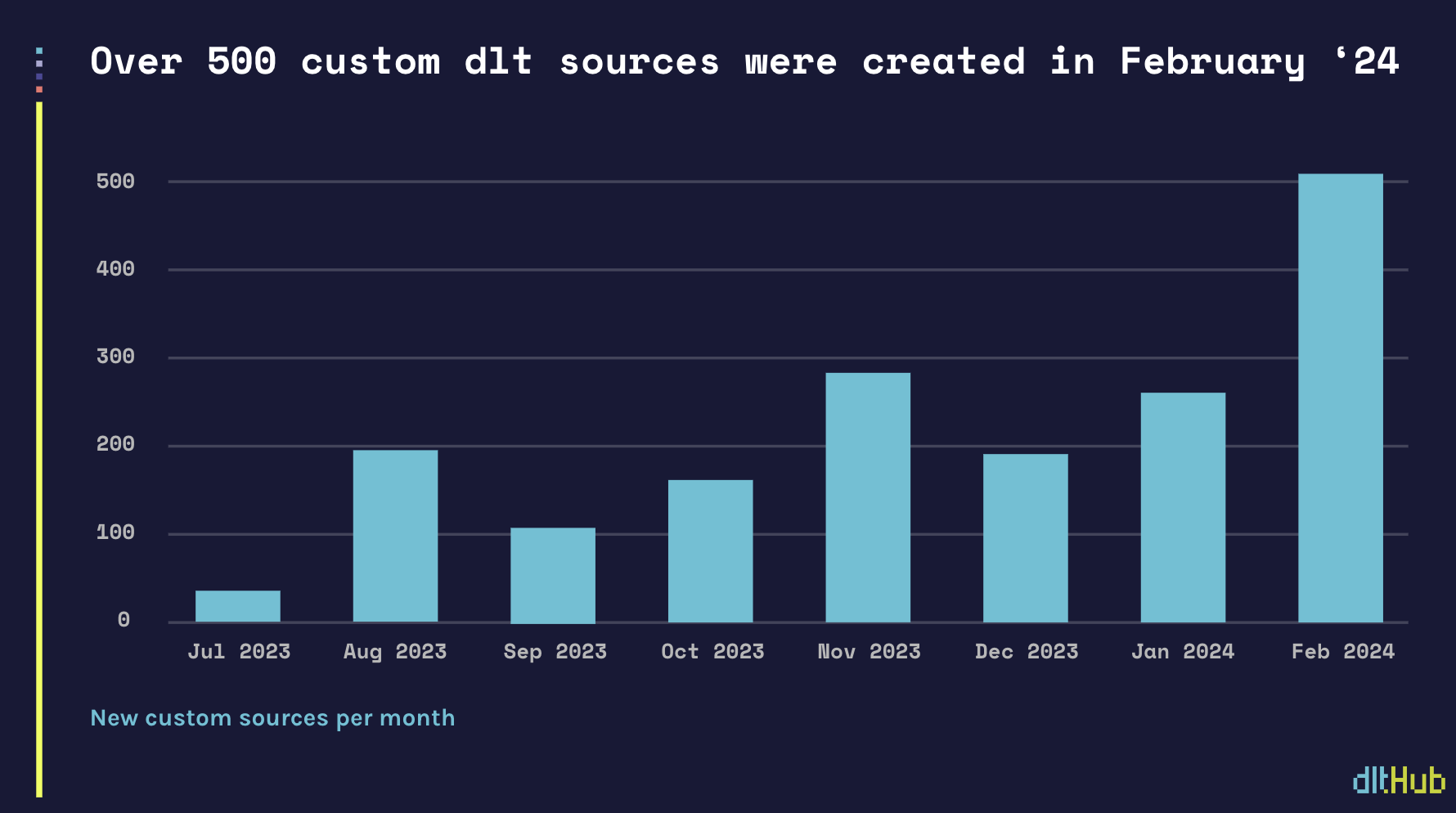
Celebrating over 500 ad hoc custom sources written by the dlt community in February

Today it is easier to pip install dlt and write a custom source than to setup and configure a traditional ETL platform.

The wider community is increasingly noticing these benefits. In February the community wrote over 500 dlt custom sources. Last week we crossed 2000 dlt total custom sources created since we launched dlt last summer.

custom sources

A custom dlt source is something new for our industry. With dlt we automated the majority of the work data engineers tasks that are usually done in traditional ETL platforms. Hence, creating an ad hoc dlt pipeline and source is a dramatically simpler. Maintaining a custom dlt source in production is relatively easy as most of the common pipeline maintenance issues are handled.

Today dlt users pick dlt because it is the fastest way to create a dataset. As we frequently hear it from all of you “dlt is pip install and go”. This is in line with our mission to make this next generation of Python users autonomous when they create and use data in their organizations.

How to get to 50,000 sources: let’s remove the dependency on source catalogs and move forward to ad hoc code

We think that “Pip install ETLs” or “EL as code” tools such as dlt are ushering a new era of ad hoc code. ad hoc code allows for automation and customization of very specific tasks.

Most of the market today is educated by Saas ETLs on the value of “source”/”connector” catalogs. The core is a short-tail catalog market of +-20 sources (product database replication, some popular CRMs and ads APIs) with the highest profit margins and intense competition among vendors. The long-tail source catalog market, depending on the vendor, is usually up to 400 sources, with much smaller support.
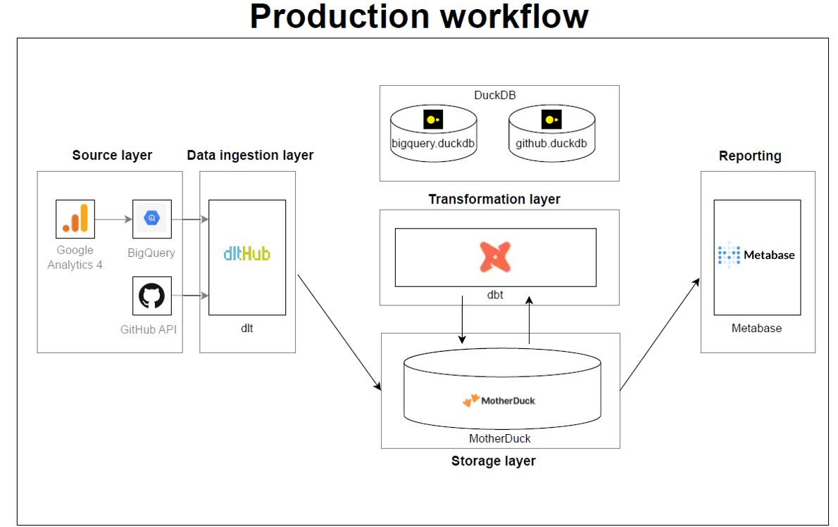
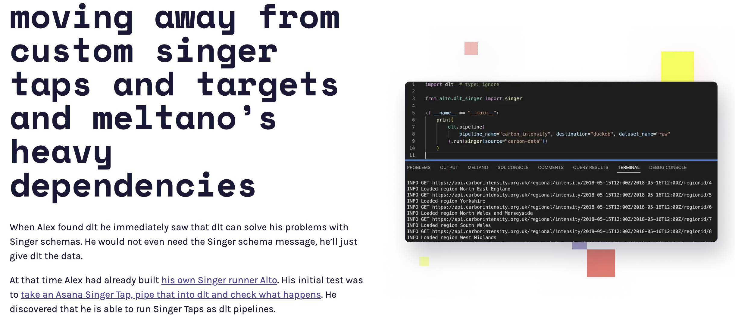
We think that source catalogs will become more and more irrelevant in the era of LLMs and ad hoc code. “EL as code” allows users to work with source catalog. From the beginning the dlt community has been writing wrappers for taps/connectors from other vendors, usually to migrate to a dlt pipeline at some point, as we documented in the customer story how Harness adopted dlt.

moving away from sources

Even for short-tail, high quality catalog sources “EL as code” allows for fixes of hidden gotchas and customisation that makes data pipelines production-ready.

We also believe that these are all early steps in “EL as code”. Huggingface hosts over 116k datasets as of March ‘24. We at dltHub think that the ‘real’ Pythonic ETL market is a market of 100k of APIs and millions of datasets.

dlt has been built for humans and LLMs from the get go and this will make coding data pipelines even faster

Since the inception of dlt, we have believed that the adoption dltamong the next generation of Python users will depend on its compatibility with code generation tools, including Codex, ChatGPT, and any new tools that emerge on the market..

We have not only been building dlt for humans, but also LLMs.

Back in March ‘23 we released dlt init as the simplest way to add a pipeline/initialize a project in dlt. We rebuilt the dlt library in such a way that it performs well with LLMs. At the end of May ‘23 we opened up our dltHub Slack to the broader community.

Back in June ‘23 we released a proof of concept of the 'dlt init' extension that can generate dlt pipelines from an OpenAPI specification. As we said at that time, if you build APIs, for example with FastAPI, you can, thanks to the OpenAPI spec, automatically generate a Python client and give it to your users. If you have 3min time watch how a demo Marcin generates such a pipeline from the OpenAPI spec using the Pokemon API in this Loom. This demo took things a step further and enables users to generate advanced dlt pipelines that, in essence, convert your API into a live dataset.

However, it takes a long time to go from a LLM PoC to production-grade code. We know much of our user base is already using ChatPGT and comparable tools to generate sources. We hear our community's excitement about the promise of LLMs for this task. The automation promise is in both in building and configuring pipelines. Anything seems possible, but if any of you have played around this task with ChatPGT - usually the results are janky. Along these lines in the last couple of months we have been dog fooding the PoC that can generate dlt pipelines from an OpenAPI specification.

comics

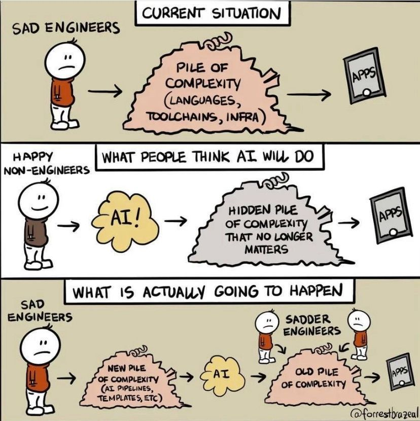
https://twitter.com/xatkit/status/1763973816798138370

You can read a case study on how our solution engineer Violetta used an iterated version of the PoC to generate a production-grade Chargebee dlt within hours instead of 2,3 days here.

We think that at this stage we are a few weeks away from releasing our next product that makes coding data pipelines faster than renting connector catalog: a dlt code generation tool that allows dlt users create datasets from the REST API in the coming weeks.

· 9 min read
Zaeem Athar
info

TL;DR: This blog post introduces a cost-effective solution for event streaming that results in up to 18x savings. The solution leverages Cloud Pub/Sub and dlt to build an efficient event streaming pipeline.

The Segment Problem

Event tracking is a complicated problem for which there exist many solutions. One such solution is Segment, which offers ample startup credits to organizations looking to set up event ingestion pipelines. Segment is used for a variety of purposes, including web analytics.

note

💡 With Segment, you pay 1-1.2 cents for every tracked users.

Let’s take a back-of-napkin example: for 100.000 users, ingesting their events data would cost $1000.

The bill:

  • Minimum 10,000 monthly tracked users (0-10K) + $120.
  • Additional 1,000 monthly tracked users (10K - 25K) + $12 / 1000 user.
  • Additional 1,000 monthly tracked users (25k - 100K) + $11 / 1000 user.
  • Additional 1,000 monthly tracked users (100k +) + $10 / 1000 user.

The price of $1000/month for 100k tracked users doesn’t seem excessive, given the complexity of the task at hand.

However, similar results can be achieved on GCP by combining different services. If those 100k users produce 1-2m events, those costs would stay in the $10-60 range.

In the following sections, we will look at which GCP services can be combined to create a cost-effective event ingestion pipeline that doesn’t break the bank.

goodbye segment

The Solution to the Segment Problem

Our proposed solution to replace Segment involves using dlt with Cloud Pub/Sub to create a simple, scalable event streaming pipeline. The pipeline's overall architecture is as follows:

pubsub_dlt-pipeline

In this architecture, a publisher initiates the process by pushing events to a Pub/Sub topic. Specifically, in the context of dlt, the library acts as the publisher, directing user telemetry data to a designated topic within Pub/Sub.

A subscriber is attached to the topic. Pub/Sub offers a push-based subscriber that proactively receives messages from the topic and writes them to Cloud Storage. The subscriber is configured to aggregate all messages received within a 10-minute window and then forward them to a designated storage bucket.

Once the data is written to the Cloud Storage this triggers a Cloud Function. The Cloud Function reads the data from the storage bucket and uses dlt to ingest the data into BigQuery.

Code Walkthrough

This section dives into a comprehensive code walkthrough that illustrates the step-by-step process of implementing our proposed event streaming pipeline.

Implementing the pipeline requires the setup of various resources, including storage buckets and serverless functions. To streamline the procurement of these resources, we'll leverage Terraform—an Infrastructure as Code (IaC) tool.

Prerequisites

Before we embark on setting up the pipeline, there are essential tools that need to be installed to ensure a smooth implementation process.

Permissions

Next, we focus on establishing the necessary permissions for our pipeline. A crucial step involves creating service account credentials, enabling Terraform to create and manage resources within Google Cloud seamlessly.

Please refer to the Google Cloud documentation here to set up a service account. Once created, it's important to assign the necessary permissions to the service account. The project README lists the necessary permissions. Finally, generate a key for the created service account and download the JSON file. Pass the credentials as environment variables in the project root directory.

export GOOGLE_APPLICATION_CREDENTIALS="/path/to/keyfile.json"

Setting Up The Event Streaming Pipeline

To set up our pipeline, start by cloning the GitHub Repository. The repository contains all the necessary components, structured as follows:

.
├── README.md
├── cloud_functions
│ ├── main.py
│ └── requirements.txt
├── publisher.py
├── requirement.txt
├── terraform
│ ├── backend.tf
│ ├── cloud_functions.tf
│ ├── main.tf
│ ├── provider.tf
│ ├── pubsub.tf
│ ├── storage_buckets.tf
│ └── variables.tf

Within this structure, the Terraform directory houses all the Terraform code required to set up the necessary resources on Google Cloud.

Meanwhile, the cloud_functions folder includes the code for the Cloud Function that will be deployed. This function will read the data from storage and use dlt to ingest data into BigQuery. The code for the function can be found in cloud_functions/main.py file.

Step 1: Configure Service Account Credentials

To begin, integrate the service account credentials with Terraform to enable authorization and resource management on Google Cloud. Edit the terraform/main.tf file to include the path to your service account's credentials file as follows:

provider "google" {
credentials = file("./../credentials.json")
project = var.project_id
region = var.region
}

Step 2: Define Required Variables

Next, in the terraform/variables.tf define the required variables. These variables correspond to details within your credentials.json file and include your project's ID, the region for resource deployment, and any other parameters required by your Terraform configuration:

variable "project_id" {
type = string
default = "Add Project ID"
}

variable "region" {
type = string
default = "Add Region"
}

variable "service_account_email" {
type = string
default = "Add Service Account Email"
}

Step 3: Procure Cloud Resources

We are now ready to set up some cloud resources. To get started, navigate into the terraform directory and terraform init. The command initializes the working directory containing Terraform configuration files.

With the initialization complete, you're ready to proceed with the creation of your cloud resources. To do this, run the following Terraform commands in sequence. These commands instruct Terraform to plan and apply the configurations defined in your .tf files, setting up the infrastructure on Google Cloud as specified.

terraform plan
terraform apply

This terraform plan command previews the actions Terraform intends to take based on your configuration files. It's a good practice to review this output to ensure the planned actions align with your expectations.

After reviewing the plan, execute the terraform apply command. This command prompts Terraform to create or update resources on Google Cloud according to your configurations.

The following resources are created on Google Cloud once terraform apply command is executed:

NameTypeDescription
tel_storageBucketBucket for storage of telemetry data.
pubsub_cfunctionsBucketBucket for storage of Cloud Function source code.
storage_bigqueryCloud FunctionThe Cloud Function that runs dlt to ingest data into BigQuery.
telemetry_data_teraPub/Sub TopicPub/Sub topic for telemetry data.
push_sub_storagePub/Sub SubscriberPub/Sub subscriber that pushes data to Cloud Storage.

Step 4: Run the Publisher

Now that our cloud infrastructure is in place, it's time to activate the event publisher. Look for the publisher.py file in the project root directory. You'll need to provide specific details to enable the publisher to send events to the correct Pub/Sub topic. Update the file with the following:

# TODO(developer)
project_id = "Add GCP Project ID"
topic_id = "telemetry_data_tera"

The publisher.py script is designed to generate dummy events, simulating real-world data, and then sends these events to the specified Pub/Sub topic. This process is crucial for testing the end-to-end functionality of our event streaming pipeline, ensuring that data flows from the source (the publisher) to our intended destinations (BigQuery, via the Cloud Function and dlt). To run the publisher execute the following command:

python publisher.py

Step 5: Results

Once the publisher sends events to the Pub/Sub Topic, the pipeline is activated. These are asynchronous calls, so there's a delay between message publication and their appearance in BigQuery.

The average completion time of the pipeline is approximately 12 minutes, accounting for the 10-minute time interval after which the subscriber pushes data to storage plus the Cloud Function execution time. The push interval of the subscriber can be adjusted by changing the max_duration in pubsub.tf

cloud_storage_config {
bucket = google_storage_bucket.tel_bucket_storage.name

filename_prefix = "telemetry-"

max_duration = "600s"

}

Our Cost Estimation

On average the cost for our proposed pipeline are as follows:

  • 100k users tracked on Segment would cost $1000.
  • 1 million events ingested via our setup $37.
  • Our web tracking user:event ratio is 1:15, so the Segment cost equivalent would be $55.
  • Our telemetry device:event ratio is 1:60, so the Segment cost equivalent would be $220.

So with our setup, as long as we keep events-to-user ratio under 270, we will have cost savings over Segment. In reality, it gets even better because GCP offers a very generous free tier that resets every month, where Segment costs more at low volumes.

GCP Cost Calculation: Currently, our telemetry tracks 50,000 anonymized devices each month on a 1:60 device-to-event ratio. Based on these data volumes we can estimate the cost of our proposed pipeline.

Cloud Functions is by far the most expensive service used by our pipeline. It is billed based on the vCPU / memory, compute time, and number of invocations.

note

💡 The cost of compute for 512MB / .333vCPU machine time for 1000ms is as follows

MetricUnit Price
GB-seconds (Memory)$0.000925
GHz-seconds (vCPU)$0.001295
Invocation$0.0000004
Total0.0022

This puts the monthly cost of ingesting 1 million events with Cloud Functions at:

  • (1 million / 60) * 0.0022 cents = $37

In Conclusion

Event streaming pipelines don’t need to be expensive. In this demo, we present an alternative to Segment that offers up to 18x in savings in practice. Our proposed solution leverages Cloud Pub/Sub and dlt to deliver a cost-effective streaming pipeline.

Following this demo requires knowledge of the publisher-subscriber model, dlt, and GCP. It took about 4 hours to set up the pipeline from scratch, but we went through the trouble and set up Terraform to procure infrastructure.

Use terraform apply to set up the needed infrastructure for running the pipeline. This can be done in 30 minutes, allowing you to evaluate the proposed solution's efficacy without spending extra time on setup. Please do share your feedback.

P.S: We will soon be migrating from Segment. Stay tuned for future posts where we document the migration process and provide a detailed analysis of the associated human and financial costs.

· 7 min read
William Laroche
info

TL;DR: William, a gcp data consultant, shares an article about the work he did with dlt and GCP to create a secure, scalable, lightweight, and powerful high-volume event ingestion engine.

He explores several alternatives before offering a solution, and he benchmarks the solution after a few weeks of running.

Read the original post here: dataroc.ca blog. Or find/hire William on Linkedin.

In the ever-evolving landscape of cloud computing, optimizing data workflows is paramount for achieving efficiency and scalability. Even though Google Cloud Platform offers the powerful Dataflow service to process data at scale, sometimes the simplest solution is worth a shot.

In cases with a relatively high Pub/Sub volume (>10 messages per second), a pull subscription with a continuously running worker is more cost-efficient and quicker than a push subscription. Using a combination of Docker, Instance Templates and Instance Groups, it is pretty simple to set up an auto-scaling group of instances that will process Pub/Sub messages.

This guide will walk you through the process of configuring GCP infrastructure that efficiently pulls JSON messages from a Pub/Sub subscription, infers schema, and inserts them directly into a Cloud SQL PostgreSQL database using micro-batch processing.

The issue at hand

In my current role at WishRoll, I was faced with the issue of processing a high amount of events and store them in the production database directly.

Imagine the scene: the server application produces analytics-style events such as "user logged-in", and "task X was completed" (among others). Eventually, for example, we want to run analytics queries on those events to count how many times a user logs in to better tailor their experience.

A. The trivial solution: synchronous insert

The trivial solution is to synchronously insert these events directly in the database. A simple implementation would mean that each event fired results in a single insert to the database. This comes with 2 main drawbacks:

  • Every API call that produces an event becomes slower. I.e. the /login endpoint needs to insert a record in the database
  • The database is now hit with a very high amount of insert queries

With our most basic need of 2 event types, we were looking at about 200 to 500 events per second. I concluded this solution would not be scalable. To make it so, 2 things would be necessary: (1) make the event firing mechanism asynchronous and (2) bulk events together before insertion.

B. The serverless asynchronous solution

A second solution is to use a Pub/Sub push subscription to trigger an HTTP endpoint when a message comes in. This would've been easy in my case because we already have a worker-style autoscaled App Engine service that could've hosted this. However, this only solves the 1st problem of the trivial solution; the events still come in one at a time to the HTTP service.

Although it's possible to implement some sort of bulking mechanism in a push endpoint, it's much easier to have a worker pull many messages at once instead.

C. The serverless, fully-managed Dataflow solution

This led me to implement a complete streaming pipeline using GCP's streaming service: Dataflow. Spoiler: this was way overkill and led to weird bugs with DLT (data load tool). If you're curious, I've open-sourced that code too.

This solved both issues of the trivial solution, but proved pretty expensive and hard to debug and monitor.

D. An autoscaled asynchronous pull worker

Disclaimer: I had never considered standalone machines from cloud providers (AWS EC2, GCP Compute Engine) to be a viable solution to my cloud problems. In my head, they seemed like outdated, manually provisioned services that could instead be replaced by managed services.

But here I was, with a need to have a continuously running worker. I decided to bite the bullet and try my luck with GCP Compute Engine. What I realized to my surprise, is that by using instance templates and instance groups, you can easily set up a cluster of workers that will autoscale.

The code is simple: run a loop forever that pulls messages from a Pub/Sub subscription, bulk the messages together, and then insert them in the database. Repeat.

Then deploy that code as an instance group that auto-scales based on the need to process messages.

Code walkthrough

The complete source code is available here.

Summarily, the code is comprised of 2 main parts:

  • The pulling and batching logic to accumulate and group messages from Pub/Sub based on their destination table
  • The load logic to infer the schema and bulk insert the records into the database. This part leverages DLT for destination compatibility and schema inference

Main loop

By using this micro-batch architecture, we strive to maintain a balance of database insert efficiency (by writing multiple records at a time) with near real-time insertion (by keeping the window size around 5 seconds).


pipeline = dlt.pipeline(
pipeline_name="pubsub_dlt",
destination=DESTINATION_NAME,
dataset_name=DATASET_NAME,
)

pull = StreamingPull(PUBSUB_INPUT_SUBCRIPTION)
pull.start()

try:
while pull.is_running:
bundle = pull.bundle(timeout=WINDOW_SIZE_SECS)
if len(bundle):
load_info = pipeline.run(bundle.dlt_source())
bundle.ack_bundle()
# pretty print the information on data that was loaded
print(load_info)
else:
print(f"No messages received in the last {WINDOW_SIZE_SECS} seconds")

finally:
pull.stop()

How to deploy

The GitHub repo explains how to deploy the project as an instance group.

Database concerns

Using DLT has the major advantage of inferring the schema of your JSON data automatically. This also comes with some caveats:

  • The output schema of these analytics tables might change based on events
  • If your events have a lot of possible properties, the resulting tables could become very wide (lots of columns) which is not something desirable in an OLTP database

Given these caveats, I make sure that all events fired by our app are fully typed and limited in scope. Moreover, using the table_name_data_key configuration of the code I wrote, it's possible to separate different events with different schemas into different tables.

See this README section for an example of application code and the resulting table.

Performance and cost

After running this code and doing backfills for a couple of weeks, I was able to benchmark the overall efficiency and cost of this solution.

Throughput capacity

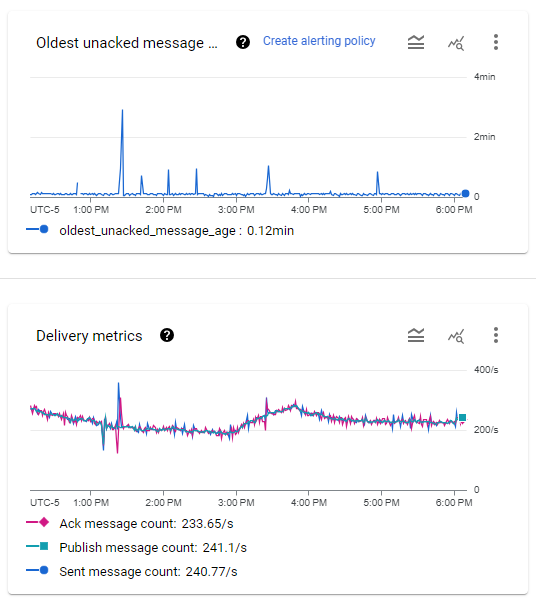
The pull worker performance

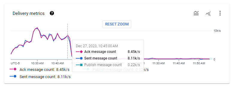
The Pub/Sub subscription metrics. Message throughput ranges between 200 and 300 per second, while the oldest message is usually between 5 and 8 seconds with occasional spikes.

I am running a preemptible (SPOT) instance group of n1-standard-1 machines that auto-scales between 2 and 10 instances. In normal operation, a single worker can handle our load easily. However, because of the preemptible nature of the instances, I set the minimum number to 2 to avoid periods where no worker is running.

Maximum capacity

When deploying the solution with a backlog of messages to process (15 hours worth of messages), 10 instances were spawned and cleared the backlog in about 25 minutes.

The Pub/Sub subscription throughput metrics when a 15-hour backlog was cleared. The instance group gradually reached 10 instances at about 10:30AM, then cleared the backlog by 10:50AM.

Between 7000 and 10000 messages per second were processed on average by these 10 instances, resulting in a minimum throughput capacity of 700 messages/s per worker.

Cost

Using n1-standard-1 spot machines, this cluster costs $8.03/mth per active machine. With a minimum cluster size of 2, this means $16.06 per month.

Conclusion

Using more "primitive" GCP services around Compute Engine provides a straightforward and cost-effective way to process a high throughput of Pub/Sub messages from a pull subscription.

info

PS from dlt team:

  • We just added data contracts enabling to manage schema evolution behavior.
  • Are you on aws? Check out this AWS SAM & Lambda event ingestion pipeline here.

· 6 min read
Anuun Chinbat

THE PROBLEM

There are two types of people: those who hoard thousands of unread emails in their inbox and those who open them immediately to avoid the ominous red notification. But one thing unites us all: everyone hates emails. The reasons are clear:

  • They're often unnecessarily wordy, making them time-consuming.
  • SPAM (obviously).
  • They become black holes of lost communication because CC/BCC-ing people doesn't always work.
  • Sometimes, there are just too many.

So, this post will explore a possible remedy to the whole email issue involving AI.


THE SOLUTION

Don't worry; it's nothing overly complex, but it does involve some cool tools that everyone could benefit from.

💡 In a nutshell, I created two flows (a main flow and a subflow) in Kestra :

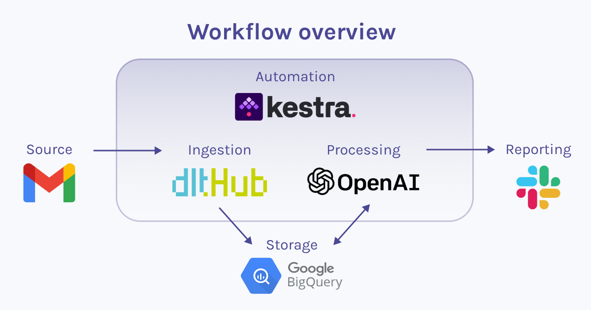
  • The main flow extracts email data from Gmail and loads it into BigQuery using dlt, checks for new emails, and, if found, triggers the subflow for further processing.
  • The subflow utilizes OpenAI to summarize and analyze the sentiment of an email, loads the results into BigQuery, and then notifies about the details via Slack.

Just so you're aware:

  • Kestra is an open-source automation tool that makes both scheduled and event-driven workflows easy.
  • dlt is an open-source library that you can add to your Python scripts to load data from various and often messy data sources into well-structured, live datasets.
tip

Wanna jump to the GitHub repo?


HOW IT WORKS

To lay it all out clearly: Everything's automated in Kestra, with hassle-free data loading thanks to dlt, and the analytical thinking handled by OpenAI. Here's a diagram to help you understand the general outline of the entire process.

overview

Now, let's delve into specific parts of the implementation.

The environment:

💡 The two flows in Kestra are set up in a very straightforward and intuitive manner. Simply follow the Prerequisites and Setup guidelines in the repo. It should take no more than 15 minutes.

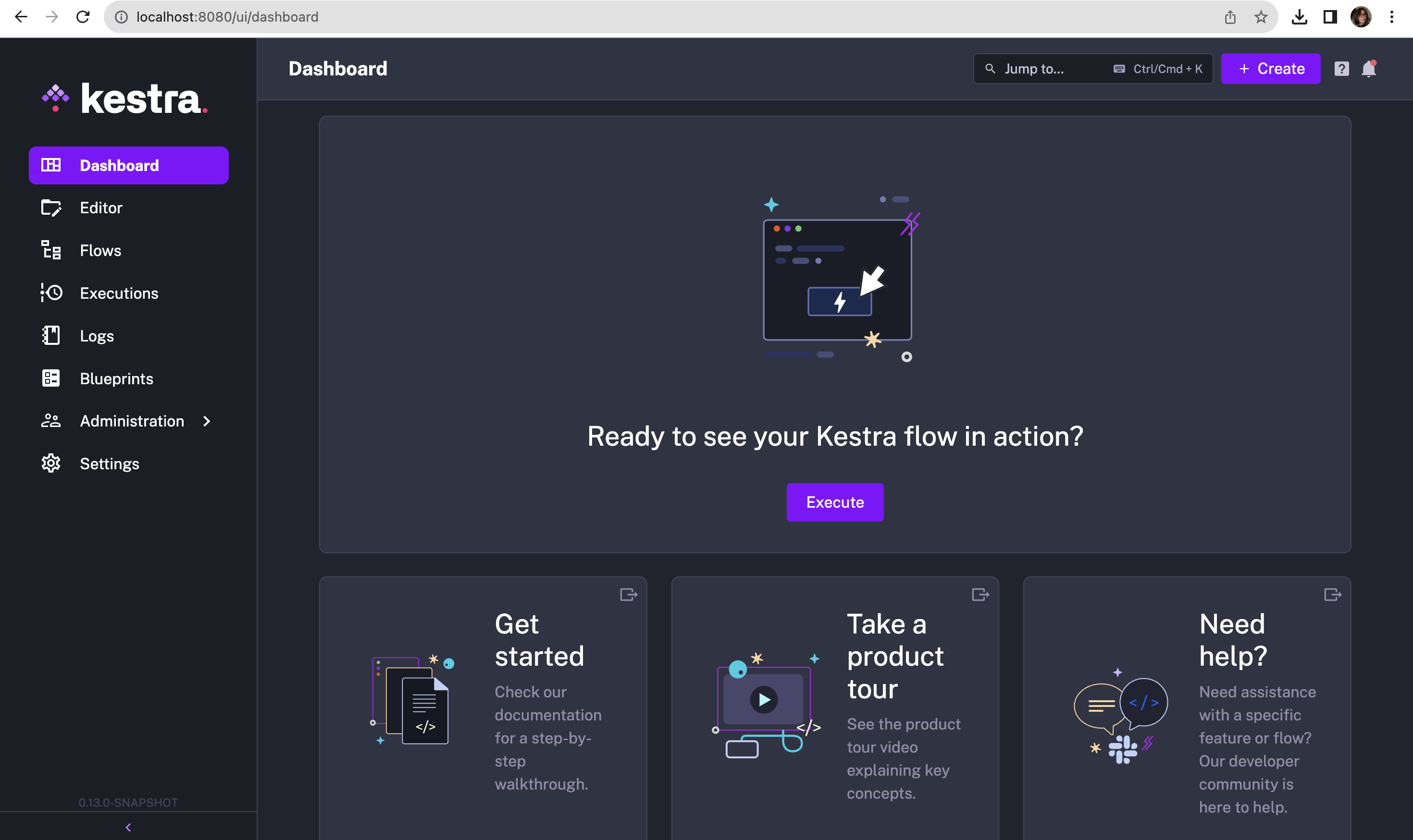
Once you’ve opened http://localhost:8080/ in your browser, this is what you’ll see on your screen:

Kestra

Now, all you need to do is create your flows and execute them.

The great thing about Kestra is its ease of use - it's UI-based, declarative, and language-agnostic. Unless you're using a task like a Python script, you don't even need to know how to code.

tip

If you're already considering ways to use Kestra for your projects, consult their documentation and the plugin pages for further insights.

The data loading part

💡 This is entirely managed by dlt in just five lines of code.

I set up a pipeline using the Inbox source – a regularly tested and verified source from dlt – with BigQuery as the destination.

In my scenario, the email data doesn't have nested structures, so there's no need for flattening. However, if you encounter nested structures in a different use case, dlt can automatically normalize them during loading.

Here's how the pipeline is defined and subsequently run in the first task of the main flow in Kestra:

# Run dlt pipeline to load email data from gmail to BigQuery
pipeline = dlt.pipeline(
pipeline_name="standard_inbox",
destination='bigquery',
dataset_name="messages_data",
dev_mode=False,
)

# Set table name
table_name = "my_inbox"
# Get messages resource from the source
messages = inbox_source(start_date = pendulum.datetime(2023, 11, 15)).messages
# Configure the messages resource to get bodies of the emails
messages = messages(include_body=True).with_name(table_name)
# Load data to the "my_inbox" table
load_info = pipeline.run(messages)

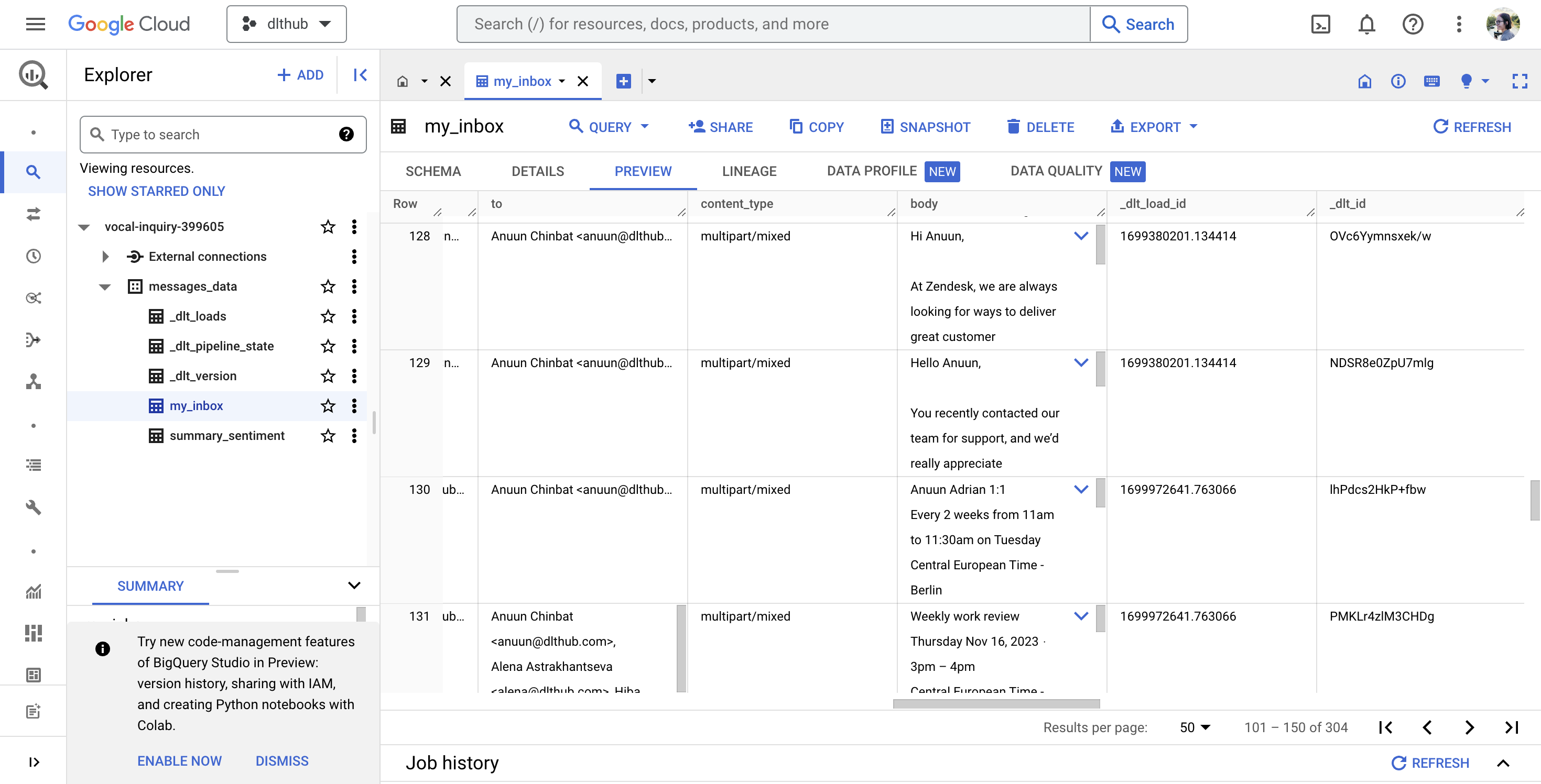
In this setup ☝️, dlt loads all email data into the table “my_inbox”, with the email body specifically stored in the “body” column. After executing your flow in Kestra, the table in BigQuery should appear as shown below:

bigquery_my_inbox

tip

This implementation doesn't handle email attachments, but if you need to analyze, for instance, invoice PDFs from your inbox, you can read about how to automate this with dlt here.

The AI part

💡 In this day and age, how can we not incorporate AI into everything? 😆

But seriously, if you're familiar with OpenAI, it's a matter of an API call to the chat completion endpoint. What simplifies it even further is Kestra’s OpenAI plugin.

In my subflow, I used it to obtain both the summary and sentiment analysis of each email body. Here's a glimpse of how it's implemented:

- id: get_summary
type: io.kestra.plugin.openai.ChatCompletion
apiKey: "{{ secret('OPENAI_API') }}"
model: gpt-3.5-turbo
prompt: "Summarize the email content in one sentence with less than 30 words: {{inputs.data[0]['body']}}"
messages: [{"role": "system", "content": "You are a tool that summarizes emails."}]
info

Kestra also includes Slack, as well as BigQuery plugins, which I used in my flows. Additionally, there is a wide variety of other plugins available.

The automation part

💡 Kestra triggers are the ideal solution!

I’ve used a schedule trigger that allows you to execute your flow on a regular cadence e.g. using a CRON expression:

triggers:
- id: schedule
type: io.kestra.core.models.triggers.types.Schedule
cron: "0 9-18 * * 1-5"

This configuration ensures that your flows are executed hourly on workdays from 9 AM to 6 PM.


THE OUTCOME

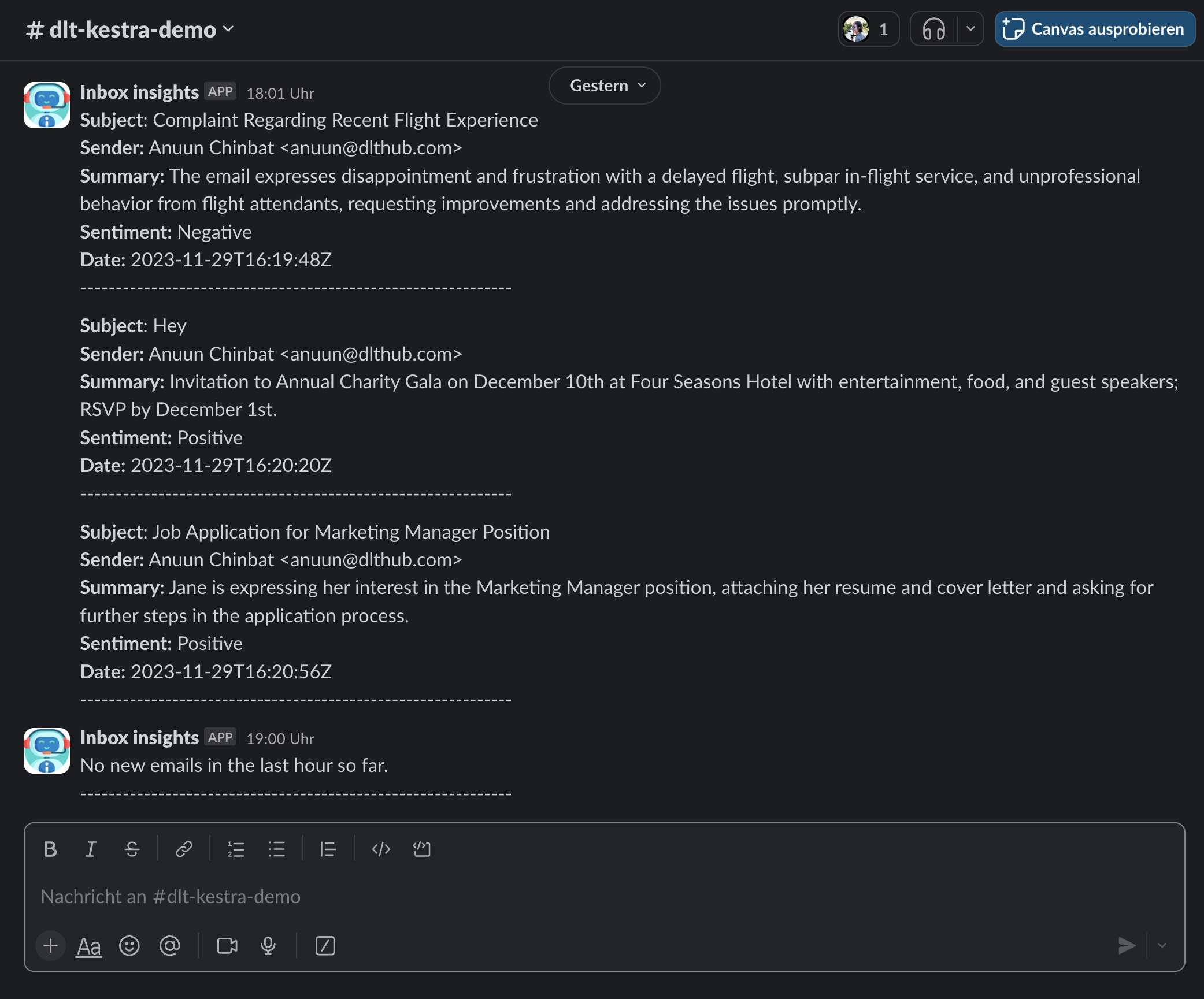
A Slack assistant that delivers crisp inbox insights right at your fingertips:

slack.png

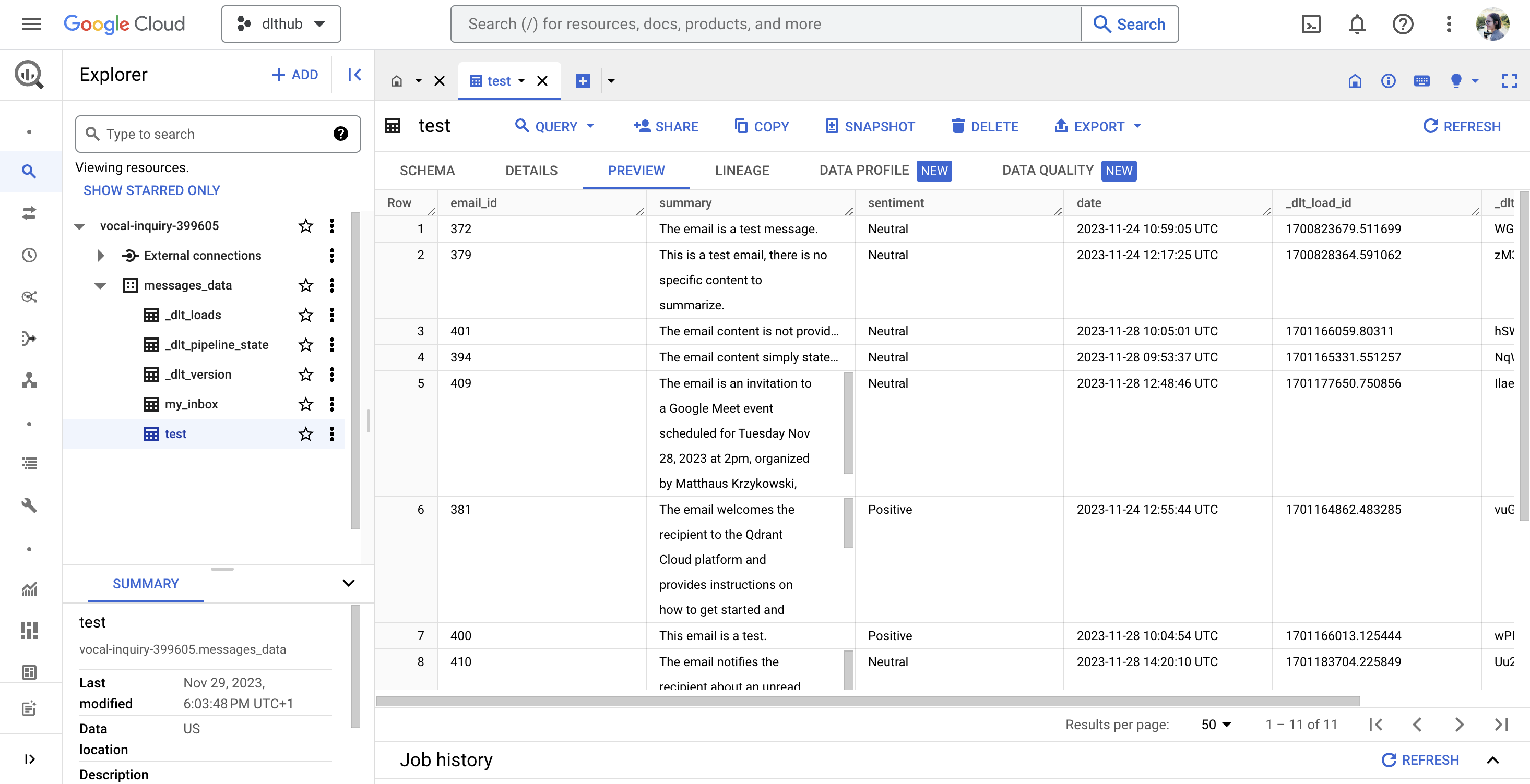
And a well-organized table in BigQuery, ready for you to dive into a more complex analysis:

bigquery_test.png

In essence, using Kestra and dlt offers a trio of advantages for refining email analysis and data workflows:

  1. Efficient automation: Kestra effortlessly orchestrates intricate workflows, integrating smoothly with tools like dlt, OpenAI, and BigQuery. This process reduces manual intervention while eliminating errors, and freeing up more time for you.
  2. User-friendly and versatile: Both Kestra and dlt are crafted for ease of use, accommodating a range of skill levels. Their adaptability extends to various use cases.
  3. Seamless scaling: Kestra, powered by Kafka and Elasticsearch, adeptly manages large-scale data and complex workflows. Coupled with dlt's solid data integration capabilities, it ensures a stable and reliable solution for diverse requirements.

HOW IT COULD WORK ELSEWHERE

Basically, you can apply the architecture discussed in this post whenever you need to automate a business process!

For detailed examples of how Kestra can be utilized in various business environments, you can explore Kestra's use cases.

Embrace automation, where the only limit is your imagination! 😛

· 9 min read
Zaeem Athar
info

TL;DR: In this blog, we'll create a data lineage view for our ingested data by utlizing the dlt load_info.

Why data lineage is important?

Data lineage is an important tool in an arsenal of a data engineer. It showcases the journey of data from its source to its destination. It captures all the pitstops made and can help identify issues in the data pipelines by offering a birds eye view of the data.

As data engineers, data lineage enables us to trace and troubleshoot the datapoints we offer to our stakeholders. It is also an important tool that can be used to meet regulation regarding privacy. Moreover, it can help us evaluate how any changes upstream in a pipeline effects the downstream source. There are many types of data lineage, the most commonly used types are the following:

  • Table lineage, it shows the raw data sources that are used to form a new table. It tracks the flow of data, showing how data moves forward through various processes and transformations.
  • Row lineage reveals the data flow at a more granular level. It refers to tracking and understanding of individual rows of data as they move through various stages in a data processing pipeline. It is a subset of table lineage that focuses specifically on the journey of individual records or rows rather than the entire dataset.
  • Column lineage specifically focuses on tracking and documenting the flow and transformation of individual columns or fields within different tables and views in the data.

Project Overview

In this demo, we showcase how you can leverage the dlt pipeline load_info to create table, row and column lineage for your data. The code for the demo is available on GitHub.

The dlt load_info encapsulates useful information pertaining the loaded data. It contains the pipeline, dataset name, the destination information and list of loaded packages among other elements. Within the load_info packages, you will find a list of all tables and columns created at the destination during loading of the data. It can be used to display all the schema changes that occur during data ingestion and implement data lineage.

We will work with the example of a skate shop that runs an online shop using Shopify, in addition to its physical stores. The data from both sources is extracted using dlt and loaded into BigQuery.

Data Lineage Overview

In order to run analytics workloads, we will create a transformed fact_sales table using dbt and the extracted raw data. The fact_sales table can be used to answer all the sales related queries for the business.

The load_info produced by dlt for both pipelines is also populated into BigQuery. We will use this information to create a Dashboard in Metabase that shows the data lineage for the fact_sales table.

Implementing Data Lineage

To get started install dlt and dbt:

pip install dlt
pip install dbt-bigquery

As we will be ingesting data into BigQuery, we first need to create service account credentials for BigQuery. You can find more info on setting up a service account in the dlt docs.

We use the following CSV files as our data sources for this demo:

dlt provides verified Shopify source to directly extract data from the Shopify API.

Step 1: Initialize a dlt pipeline

To get started we initialize a dlt pipeline and selecting BigQuery as our destination by running the following command:

dlt init data_lineage bigquery

This will create default scaffolding to build our pipeline. Install the dependencies by running the following command:

pip install -r requirements.txt

Loading the data

As a first step, we will load the sales data from the online and physical store of the skate shop into BigQuery. In addition to the sales data, we will also ingest the dlt load_info into BigQuery. This will help us track changes in our pipeline.

Step 2: Adding the dlt pipeline code

In the data_lineage.py file remove the default code and add the following:

FILEPATH = "data/supermarket_sales.csv"
FILEPATH_SHOPIFY = "data/orders_export_1.csv"

class Data_Pipeline:
def __init__(self, pipeline_name, destination, dataset_name):
self.pipeline_name = pipeline_name
self.destination = destination
self.dataset_name = dataset_name

def run_pipeline(self, data, table_name, write_disposition):
# Configure the pipeline with your destination details
pipeline = dlt.pipeline(
pipeline_name=self.pipeline_name,
destination=self.destination,
dataset_name=self.dataset_name
)
# Run the pipeline with the provided data
load_info = pipeline.run(
data,
table_name=table_name,
write_disposition=write_disposition
)

# Pretty print the information on data that was loaded
print(load_info)
return load_info

Any changes in the underlying data are captured by the dlt load_info. To showcase this, we will filter the data to remove the Branch and Tags columns from Store and Shopify data respectively and run the pipeline. Later we will add back the columns and rerun the pipeline. These new columns added will be recorded in the load_info packages.

We will add the load_info back to BigQuery to use in our Dashboard. The Dashboard will provide an overview data lineage for our ingested data.

if __name__ == "__main__":

data_store = pd.read_csv(FILEPATH)
data_shopify = pd.read_csv(FILEPATH_SHOPIFY)

#filtering some data.
select_c_data_store = data_store.loc[
:, data_store.columns.difference(['Branch'])
]
select_c_data_shopify = data_shopify.loc[
:, data_shopify.columns.difference(['Tags'])
]

pipeline_store = Data_Pipeline(
pipeline_name='pipeline_store',
destination='bigquery',
dataset_name='sales_store'
)
pipeline_shopify = Data_Pipeline(
pipeline_name='pipeline_shopify',
destination='bigquery',
dataset_name='sales_shopify'
)

load_a = pipeline_store.run_pipeline(
data=select_c_data_store,
table_name='sales_info',
write_disposition='replace'
)
load_b = pipeline_shopify.run_pipeline(
data=select_c_data_shopify,
table_name='sales_info',
write_disposition='replace'
)

pipeline_store.run_pipeline(
data=load_a.load_packages,
table_name="load_info",
write_disposition="append"
)
pipeline_shopify.run_pipeline(
data=load_b.load_packages,
table_name='load_info',
write_disposition="append"
)

Step 3: Run the dlt pipeline

To run the pipeline, execute the following command:

python data_lineage.py

This will load the data into BigQuery. We now need to remove the column filters from the code and rerun the pipeline. This will add the filtered columns to the tables in BigQuery. The change will be captured by dlt.

Data Transformation and Lineage

Now that both the Shopify and Store data are available in BigQuery, we will use dbt to transform the data.

Step 4: Initialize a dbt project and define model

To get started initialize a dbt project in the root directory:

dbt init sales_dbt

Next, in the sales_dbt/models we define the dbt models. The first model will be the fact_sales.sql. The skate shop has two data sources: the online Shopify source and the physical Store source. We need to combine the data from both sources to create a unified reporting feed. The fact_sales table will be our unified source.

Code for fact_sales.sql:

{{ config(materialized='table') }}

select
invoice_id,
city,
unit_price,
quantity,
total,
date,
payment,
info._dlt_id,
info._dlt_load_id,
loads.schema_name,
loads.inserted_at
from {{source('store', 'sales_info')}} as info
left join {{source('store', '_dlt_loads')}} as loads
on info._dlt_load_id = loads.load_id

union all

select
name as invoice_id,
billing_city,
lineitem_price,
lineitem_quantity,
total,
created_at,
payment_method,
info._dlt_id,
info._dlt_load_id,
loads.schema_name,
loads.inserted_at
from {{source('shopify', 'sales_info')}} as info
left join {{source('shopify', '_dlt_loads')}} as loads
on info._dlt_load_id = loads.load_id
where financial_status = 'paid'

In the query, we join the sales information for each source with its dlt load_info. This will help us keep track of the number of rows added with each pipeline run. The schema_name identifies the source that populated the table and helps establish the table lineage. While the _dlt_load_id identifies the pipeline run that populated the each row and helps establish row level lineage. The sources are combined to create a fact_sales table by doing a union over both sources.

Next, we define the schema_change.sql model to capture the changes in the table schema using a following query:

{{ config(materialized='table') }}

select *
from {{source('store', 'load_info__tables__columns')}}

union all

select *
from {{source('shopify', 'load_info__tables__columns')}}

In the query, we combine the load_info for both sources by doing a union over the sources. The resulting schema_change table contains records of the column changes that occur on each pipeline run. This will help us track the column lineage and will be used to create our Data Lineage Dashboard.

Step 5: Run the dbt package

In the data_lineage.py add the code to run the dbt package using dlt.

pipeline_transform = dlt.pipeline(
pipeline_name='pipeline_transform',
destination='bigquery',
dataset_name='sales_transform'
)

venv = Venv.restore_current()
here = os.path.dirname(os.path.realpath(__file__))

dbt = dlt.dbt.package(
pipeline_transform,
os.path.join(here, "sales_dbt/"),
venv=venv
)

models = dbt.run_all()

for m in models:
print(
f"Model {m.model_name} materialized in {m.time} - "
f"Status {m.status} and message {m.message}"
)

Next, run the pipeline using the following command:

python data_lineage.py

Once the pipeline is run, a new dataset called sales_transform will be created in BigQuery, which will contain the fact_sales and schema_changes tables that we defined in the dbt package.

Step 6: Visualising the lineage in Metabase

To access the BigQuery data in Metabase, we need to connect BigQuery to Metabase. Follow the Metabase docs to connect BigQuery to Metabase.

Once BigQuery is connected with Metabase, use the SQL Editor to create the first table. The Data Load Overview table gives an overview of the dlt pipelines that populated the fact_sales table. It shows the pipeline names and the number of rows loaded into the fact_sales table by each pipeline.

Metabase Report

This can be used to track the rows loaded by each pipeline. An upper and lower threshold can be set, and when our pipelines add rows above or below the threshold, that can act as our canary in the coal mine.

Next, we will visualize the fact_sales and the schema_changes as a table and add the dlt_load_id as a filter. The resulting Data Lineage Dashboard will give us an overview of the table, row and column level lineage for our data.

Data Lineage Dashboard

When we filter by the dlt_load_id the dashboard will filter for the specific pipeline run. In the Fact Sales table the column schema_name identifies the raw sources that populated the table (Table lineage). The table also shows only the rows that were added for the pipeline run (Row Lineage). Lastly, the Updated Columns table revels the columns that were added for filtered pipeline run (Column Lineage).

When we ran the pipeline initially, we filtered out the Tags column and later reintroduced it and ran the pipeline again. The Updated Columns shows that the Tags column was added to the Fact Sales table with the new pipeline run.

Conclusion

Data lineage provides an overview of the data journey from the source to destination. It is an important tool that can help troubleshoot a pipeline. dlt load_info provides an alternative solution to visualizing data lineage by tracking changes in the underlying data.

Although dlt currently does not support data flow diagrams, it tracks changes in the data schema that can be used to create dashboards that provides an overview of table, row and column lineage for the loaded data.

· 11 min read
Zaeem Athar
info

TL;DR: In this blog post, we'll build data piplines using dlt and orchestrate them using Dagster.

dlt is an open-source Python library that allows you to declaratively load messy data sources into well-structured tables or datasets, through automatic schema inference and evolution. It simplifies building data pipelines by providing functionality to support the entire extract and load process.

It does so in a scalable way, enabling you to run it on both micro workers or in highly parallelized setups. dlt also offers robustness on extraction by providing state management for incremental extraction, drop-in requests replacement with retries, and many other helpers for common and uncommon extraction cases.

To start with dlt, you can install it using pip: pip install dlt. Afterward, import dlt in your Python script and start building your data pipeline. There's no need to start any backends or containers.

Project Overview:

In this example, we will ingest GitHub issue data from a repository and store the data in BigQuery. We will use dlt to create a data pipeline and orchestrate it using Dagster.

Initially, we will start by creating a simple data pipeline using dlt. We will then orchestrate the pipeline using Dagster. Finally, we will add more features to this pipeline by using the dlt schema evolution and Dagster asset metadata to educate the users about their data pipeline.

The project code is available on GitHub.

Project Overview

As we will be ingesting data into BigQuery we first need to create service account credentials for BigQuery. You can find more info on setting up a service account in the dlt docs.

Once we have the credentials we are ready to begin. Let’s first install Dagster and dlt. The below commands should install both.

pip install dlt
pip install dagster dagster-webserver

Simple dlt Pipeline:

As a first step, we will create the GitHub issues pipeline using dlt.

dlt init github_issues bigquery

This will generate a template for us to create a new pipeline. Under .dlt/secrets.toml add the service account credentials for BigQuery. Then in the github_issues.py delete the generated code and add the following:

@dlt.resource(write_disposition="append")
def github_issues_resource(api_secret_key=dlt.secrets.value):
owner = 'dlt-hub'
repo = 'dlt'
url = f"https://api.github.com/repos/{owner}/{repo}/issues"
headers = {"Accept": "application/vnd.github.raw+json"}

while url:
response = requests.get(url, headers=headers)
response.raise_for_status() # raise exception if invalid response
issues = response.json()
yield issues

if 'link' in response.headers:
if 'rel="next"' not in response.headers['link']:
break

url = response.links['next']['url'] # fetch next page of stargazers
else:
break
time.sleep(2) # sleep for 2 seconds to respect rate limits

if __name__ == "__main__":
# configure the pipeline with your destination details
pipeline = dlt.pipeline(
pipeline_name='github_issues', destination='bigquery', dataset_name='github_issues_data'
)

# run the pipeline with your parameters
load_info = pipeline.run(github_issues_resource())

#print the information on data that was loaded
print(load_info)

The above code creates a simple github_issues pipeline that gets the issues data from the defined repository and loads it into BigQuery. The dlt.resources yields the data while the dlt.pipeline normalizes the nested data and loads it into the defined destination. To read more about the technical details refer to the dlt docs.

To run the pipeline execute the below commands:

pip install -r requirements.txt
python github_issues.py

We now have a running pipeline and are ready to orchestrate it using Dagster.

Orchestrating using Dagster:

We will need to adjust our pipeline a bit to orchestrate it using Dagster.

Step 1: Create a Dagster project

  • Create a new directory for your Dagster project and scaffold the basic structure:
mkdir dagster_github_issues
cd dagster_github_issues
dagster project scaffold --name github-issues

This will generate the default files for Dagster that we will use as a starting point for our data pipeline.

Step 2: Set up the directory structure

  • Inside the github-issues/github_issues directory create the following folders: assets, resources, and dlt.
.
├── README.md
├── github_issues
│ ├── __init__.py
│ ├── assets
│ │ ├── __init__.py
│ ├── dlt
│ │ ├── __init__.py
│ └── resources
│ ├── __init__.py
├── github_issues_tests
│ ├── __init__.py
│ └── test_assets.py
├── pyproject.toml
├── setup.cfg
└── setup.py

Step 3: Add dlt Resources and environment variables

  • Copy the previously created github_issues_resource code into dlt/__init__.py under the dlt folder. Remove the dlt.secrets.value parameter, as we'll pass the credentials through a .env file.
  • Create a .env file in the root directory. This is the directory where the pyproject.toml file exits. Copy the credentials into the .env and follow the correct naming convention. For more info on setting up the .env file have a look at the docs.

Step 4: Add configurable resources and define the asset

  • Define a DDltResource class in resources/__init__.py as a Dagster configurable resource. This class allows you to reuse pipeline code inside an asset.
from dagster import ConfigurableResource 
import dlt

class DDltResource(ConfigurableResource):
pipeline_name: str
dataset_name: str
destination: str

def create_pipeline(self, resource_data, table_name):

# configure the pipeline with your destination details
pipeline = dlt.pipeline(
pipeline_name=self.pipeline_name, destination=self.destination, dataset_name=self.dataset_name
)

# run the pipeline with your parameters
load_info = pipeline.run(dlt_resource, table_name=table_name)

return load_info
  • Define the asset, issues_pipeline, in assets/__init__.py. This asset uses the configurable resource to create a dlt pipeline and ingests data into BigQuery.
from dagster import asset, get_dagster_logger
from ..resources import DDltResource
from ..dlt import github_issues_resource

@asset
def issues_pipeline(pipeline: DDltResource):

logger = get_dagster_logger()
results = pipeline.create_pipeline(github_issues_resource, table_name='github_issues')
logger.info(results)

The defined asset (issues_pipeline) takes as input the configurable resource (DDltResource). In the asset, we use the configurable resource to create a dlt pipeline by using an instance of the configurable resource (DDltResource) to call the create_pipeline function. The dlt.resource (github_issues_resource) is passed to the create_pipeline function. The create_pipeline function normalizes the data and ingests it into BigQuery.

Step 5: Handle Schema Evolution

dlt provides the feature of schema evolution that monitors changes in the defined table schema. Suppose GitHub adds a new column or changes a datatype of a column this small change can break pipelines and transformations. The schema evolution feature works amazingly well with Dagster.

  • Add the schema evolution code to the asset to make our pipelines more resilient to changes.
from dagster import AssetExecutionContext
@asset
def issues_pipeline(context: AssetExecutionContext, pipeline: DDltResource):
...
md_content=""
for package in result.load_packages:
for table_name, table in package.schema_update.items():
for column_name, column in table["columns"].items():
md_content= f"\tTable updated: {table_name}: Column changed: {column_name}: {column['data_type']}"

# Attach the Markdown content as metadata to the asset
context.add_output_metadata(metadata={"Updates": MetadataValue.md(md_content)})

Step 6: Define Definitions

  • In the __init.py__ under the github_issues folder add the definitions:
all_assets = load_assets_from_modules([assets])
simple_pipeline = define_asset_job(name="simple_pipeline", selection= ['issues_pipeline'])

defs = Definitions(
assets=all_assets,
jobs=[simple_pipeline],
resources={
"pipeline": DDltResource(
pipeline_name = "github_issues",
dataset_name = "dagster_github_issues",
destination = "bigquery",
table_name= "github_issues"
),
}
)

Step 7: Run the Web Server and materialize the asset

  • In the root directory (github-issues) run the dagster dev command to run the web server and materialize the asset.

GitHub Asset

Step 8: View the populated Metadata and ingested data in BigQuery

Once the asset has been successfully materialized go to the Assets tab from the top and select the Issues_pipeline. In the Metadata you can see the Tables, Columns, and Data Types that have been updated. In this case, the changes are related to internal dlt tables.

Any subsequent changes in the GitHub issues schema can be tracked from the metadata. You can set up Slack notifications to be alerted to schema changes.

Meatadata loaded in Asset

Let's finally have a look in BigQuery to view the ingested data.

Data Loaded in Bigquery

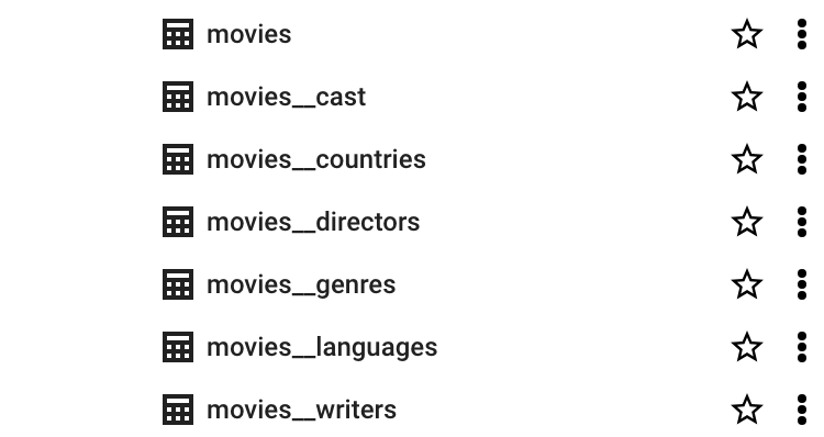
The github_issues is the parent table that contains the data from the root level of the JSON returned by the GitHub API. The subsequent table github_issues_assignees is a child table that was nested in the original JSON. dlt normalizes nested data by populating them in separate tables and creates relationships between the tables. To learn more about how dlt created these relationships refer to the docs.

Orchestrating verified dlt source using Dagster:

dlt provides a list of verified sources that can be initialized to fast-track the pipeline-building process. You can find a list of sources provided in the dlt docs.

One of the main strengths of dlt lies in its ability to extract, normalize, and ingest unstructured and semi-structured data from various sources. One of the most commonly used verified source is MongoDB. Let’s quickly look at how we can orchestrate MongoDB source using Dagster.

Step 1: Setting up a Dagster project

  • Start by creating a new Dagster project scaffold:
dagster project scaffold --name mongodb-dlt
  • Follow the steps mentioned earlier and create an assets, and resources directory under mongodb-dlt/mongodb_dlt.
  • Initialize a dlt MongoDB pipeline in the same directory:
dlt init mongodb bigquery

This will create a template with all the necessary logic implemented for extracting data from MongoDB. After running the command your directory structure should be as follows:

.
├── README.md
├── mongodb_dlt
│ ├── __init__.py
│ ├── assets
│ │ ├── __init__.py
│ │ └── assets.py
│ ├── mongodb
│ │ ├── README.md
│ │ ├── __init__.py
│ │ └── helpers.py
│ ├── mongodb_pipeline.py
│ ├── requirements.txt
│ └── resources
│ ├── __init__.py
├── mongodb_dlt_tests
│ ├── __init__.py
│ └── test_assets.py
├── pyproject.toml
├── setup.cfg
└── setup.py

Step 2: Configuring MongoDB Atlas and Credentials

For this example, we are using MongoDB Atlas. Set up the account for MongoDB Atlas and use the test Movie Flix Dataset. You can find detailed information on setting up the credentials in the MongoDB verified sources documentation.

Next, create a .env file and add the BigQuery and MongoDB credentials to the file. The .env file should reside in the root directory.

Step 3: Adding the DDltResource

Create a DltResouce under the resources directory. Add the following code to the __init__.py:

from dagster import ConfigurableResource 

import dlt

class DDltResource(ConfigurableResource):
pipeline_name: str
dataset_name: str
destination: str

def load_collection(self, resource_data, database):

# configure the pipeline with your destination details
pipeline = dlt.pipeline(
pipeline_name=f"{database}_{self.pipeline_name}", destination=self.destination, dataset_name=f"{self.dataset_name}_{database}"
)

load_info = pipeline.run(resource_data, write_disposition="replace")

return load_info

Step 4: Defining an Asset Factory

The structure of data in MongoDB is such that under each database you will find multiple collections. When writing a data pipeline it is important to separate the data loading for each collection.

Dagster provides the feature of @multi_asset declaration that will allow us to convert each collection under a database into a separate asset. This will make our pipeline easy to debug in case of failure and the collections independent of each other.

In the mongodb_pipeline.py file, locate the load_select_collection_hint_db function. We will use this function to create the asset factory.

In the __init__.py file under the assets directory, define the dlt_asset_factory:

from ..mongodb import mongodb
from ..resources import DDltResource

import dlt
import os

URL = os.getenv('SOURCES__MONGODB__CONNECTION__URL')

DATABASE_COLLECTIONS = {
"sample_mflix": [
"comments",
"embedded_movies",
],
}

def dlt_asset_factory(collection_list):
multi_assets = []

for db, collection_name in collection_list.items():
@multi_asset(
name=db,
group_name=db,
outs={
stream: AssetOut(key_prefix=[f'raw_{db}'])
for stream in collection_name}

)
def collections_asset(context: OpExecutionContext, pipeline: DDltResource):

# Getting Data From MongoDB
data = mongodb(URL, db).with_resources(*collection_name)

logger = get_dagster_logger()
results = pipeline.load_collection(data, db)
logger.info(results)

return tuple([None for _ in context.selected_output_names])

multi_assets.append(collections_asset)

return multi_assets


dlt_assets = dlt_asset_factory(DATABASE_COLLECTIONS)

Step 5: Definitions and Running the Web Server

Add the definitions in the __init__.py in the root directory:

from dagster import Definitions

from .assets import dlt_assets
from .resources import DDltResource

defs = Definitions(
assets=dlt_assets,
resources={
"pipeline": DDltResource(
pipeline_name = "mongo",
dataset_name = "dagster_mongo",
destination = "bigquery"
),
}
)

We can run the dagster dev command to start the web server. We can see that each collection is converted into a separate asset by Dagster. We can materialize our assets to ingest the data into BigQuery.

Asset Factory

The resulting data in BigQuery:

Data Ingestion in BigQuery from MongoDB

Conclusion:

In this demo, we looked at how to orchestrate dlt pipelines using Dagster. We started off by creating a simple dlt pipeline and then converted the pipeline into an asset and resource before orchestrating.

We also looked at how we can orchestrate dlt MongoDB verified sources using Dagster. We utilized the Dagster @multi_asset feature to create a dlt_asset_factory which converts each collection under a database to a separate asset allowing us to create more robust data pipelines.

Both dlt and Dagster can be easily run on local machines. By combining the two we can build data pipelines at great speed and rigorously test them before shipping to production.

· 19 min read
Zaeem Athar
info

TL;DR: A modern analytics stack with dlt and Holistics to transform and ingest unstructured production data from MongoDB to flat tables in BigQuery for self-service analytics.

If you’re a CTO, then you probably love MongoDB: it’s scalable, production-ready, and a great dump for unstructured, and semi-structured data. If you’re however a data scientist or data analyst and you need to run analytics on top of MongoDB data dumps, then you’re probably not a fan. The data in MongoDB needs to be transformed and stored in a data warehouse before it is ready for analytics. The process of transforming and storing the data can become quite tedious due to the unstructured nature of the data.

In this blog, we will show you how you can combine dlt and Holistics and create a modern data stack that makes the process of extracting unstructured data from MongoDB, and running self-service analytics on the data simple and straightforward. We will use dlt to ingest the Movie Flix Dataset into BigQuery from MongoDB and use Holistics to transform the data and run self-service analytics.

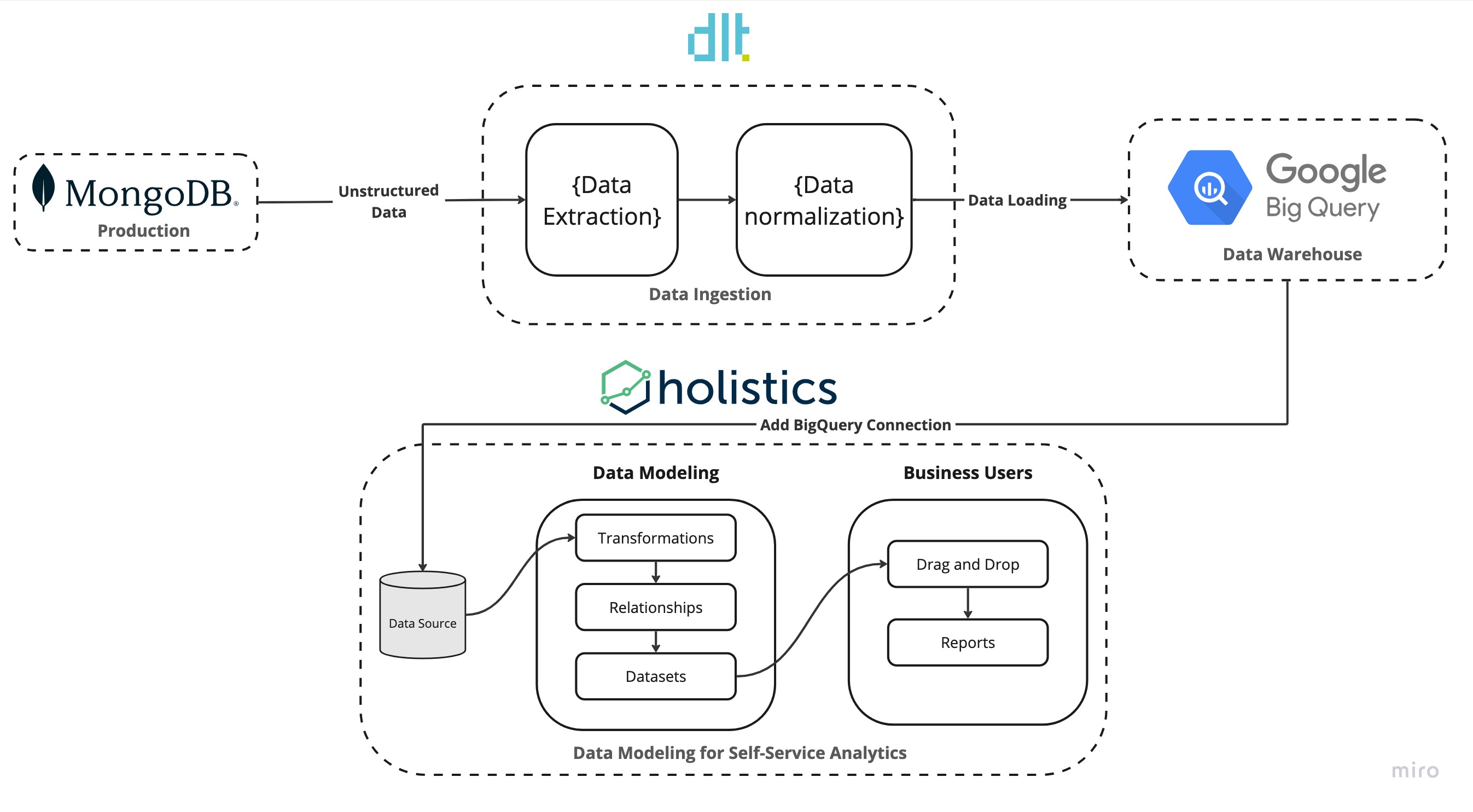
An Overview of the MongoDB Modern Analytics Stack

Diagram illustrating the inner workings of our Modern Analytics Stack

ToolLayerWhy it’s awesome
MongoDBProductionSometimes used as a data dump by CTOs. Often stores unstructured, semi-structured production data that stakeholders want to access.
dltData IngestionMongo is great, but then others struggle to analyze the data. dlt extracts data from MongoDB, creates schema in BigQuery, and loads normalized MongoDB data into BigQuery.
BigQueryData WarehouseBecause of its pricing model, it’s a good data warehouse choice to store structured MongoDB data so it can be used by BI tools like Holistics for self-service analytics.
HolisticsData Modeling for Self-Service AnalyticsHolistics makes it easy for data teams to setup and govern an end-user self-service analytics platform using DevOps best practices

In our stack, dlt resides in the data ingestion layer. It takes in unstructured data from MongoDB normalizes the data and populates it into BigQuery.

In the data modeling layer, Holistics accesses the data from BigQuery builds relationships, transforms the data, and creates datasets to access the transformations. In the reporting layer, Holistics allows stakeholders to self-service their data by utilizing the created datasets to build reports and create visualizations.

MongoDB is loved by CTOs, but its usage creates issues for stakeholders.

NoSQL databases such as MongoDB have gained widespread popularity due to their capacity to store data in formats that align more seamlessly with application usage, necessitating fewer data transformations during storage and retrieval.

MongoDB is optimized for performance and uses BSON (Binary Javascript Object Notation) under the hood as compared to JSON. This allows MongoDB to support custom and more complex data types, such as geospatial data, dates, and regex. Additionally, BSON supports character encodings.

All these benefits enable MongoDB to be a faster and better database, but the advantages of the flexibility offered by MongoDB are sometimes abused by developers and CTOs who use it as a dump for all types of unstructured and semi-structured data. This makes this data inaccessible to stakeholders and unfit for analytics purposes.

Moreover, the unique nature of MongoDB with its BSON types and its usage as a data dump in current times mean that additional hurdles must be crossed before data from MongoDB can be moved elsewhere.

How does our Modern data stack solve the MongoDB problem?

In the data ingestion layer, dlt utilizes the MongoDB verified source to ingest data into BigQuery. Initializing the MongoDB verified source setups default code needed to run the pipeline. We just have to setup the credentials and specify the collections in MongoDB to ingest into BigQuery. Once the pipeline is run dlt takes care of all the steps from extracting unstructured data from MongoDB, normalizing the data, creating schema, and populating the data into BigQuery.

Getting your data cleaned and ingested into a data warehouse is just one part of the analytics pipeline puzzle. Before the data is ready to be used by the entire organization the data team must model the data and document the context of data. This means defining the relationships between tables, adding column descriptions, and implementing the necessary transformations. This is where Holistics shines. With analytics-as-code as first-class citizens, Holistics allows data teams to adopt software engineering best practices in their analytics development workflows. This helps data teams govern a centralized curated set of semantic datasets that any business users can use to extract data from the data warehouse.

Why is dlt useful when you want to ingest data from a production database such as MongoDB?

Writing a Python-based data ingestion pipeline for sources such as MongoDB is quite a tedious task as it involves a lot of overhead to set up. The data needs to be cleaned before it is ready for ingestion. Moreover, MongoDB is a NoSQL database meaning it stores data in a JSON-like data structure. So if you want to query it with SQL natively, you will need to transform this JSON-like data structure into flat tables. Let's look at how this transformation and cleaning can be done:

  • Create a Data Model based on the MongoDB data we intend to ingest.
  • Create tables in the data warehouse based on the defined Data Model.
  • Extract the data from MongoDB and perform necessary transformations such as Data Type conversion (BSON to JSON), and flattening of nested data.
  • Insert the transformed data into the corresponding SQL tables.
  • Define relationships between tables by setting up primary and foreign keys.

Using the dlt MongoDB verified source we can forgo the above-mentioned steps. dlt takes care of all the steps from transforming the JSON data into relational data, to creating the schema in the SQL database.

To get started with dlt we would need to set some basic configurations, while everything else would be automated. dlt takes care of all the steps from creating schema to transforming the JSON data into relational data. The workflow for creating such a data pipeline in dlt would look something like this:

  • Initialize a MongoDB source to copy the default code.
  • Set up the credentials for the source and destination.
  • Define the MongoDB collection to ingest (or default to all).
  • Optionally configure incremental loading based on source logic.

What is useful about Holistics in this project?

Holistics is a Business Intelligence platform with the goal of enabling self-service analytics for entire organizations. Holistics works by connecting to an SQL data warehouse. This allows it to build SQL queries and execute them against the data warehouse. In essence, Holistics utilizes the storage and processing capabilities of the data warehouse and the data never leaves the data warehouse.

To enable self-service Holistics introduces a modeling layer. The data teams use this layer to define table relationships, data transformations, metrics, and data logic. The entire organization can utilize these metrics and data logic defined in this layer to self-service their data needs.

In addition to the transformation layer, Holistics provides advanced features such as defining models using code through Holistics’ analytics-as-code languages (AMQL) and utilizing Git version control systems to manage code changes. Moreover, data teams can integrate with dbt to streamline the data transformations.

The overall Holistics workflow looks something like this:

Holistics Overview

  • Connect Holistics to an existing SQL data warehouse.
  • Data teams use Holistics Data Modeling to model and transform analytics data. This model layer is reusable across reports & datasets.
  • Non-technical users can self-service explore data based on predefined datasets prepared by data teams. They can save their explorations into dashboards for future use.
  • Dashboards can be shared with others, or pushed to other platforms (email, Slack, webhooks, etc.).

Code Walkthrough

In this section, we walk through how to set up a MongoDB data pipeline using dlt. We will be using the MongoDB verified source you can find here.

1. Setting up the dlt pipeline

Use the command below to install dlt.

pip3 install -U dlt

Consider setting up a virtual environment for your projects and installing the project-related libraries and dependencies inside the environment. For best installation practices visit the dlt installation guide.

Once we have dlt installed, we can go ahead and initialize a verified MongoDB pipeline with the destination set to Google BigQuery. First, create a project directory and then execute the command below:

dlt init mongodb bigquery

The above command will create a local ready-made pipeline that we can customize to our needs. After executing the command your project directory will look as follows:

.
├── .dlt
│ ├── config.toml
│ └── secrets.toml
├── mongodb
│ ├── README.md
│ ├── __init__.py
│ └── helpers.py
├── mongodb_pipeline.py
└── requirements.txt

The __init__.py file in the mongodb directory contains dlt functions we call resources that yield the data from MongoDB. The yielded data is passed to a dlt.pipeline that normalizes the data and forms the connection to move the data to your destination. To get a better intuition of the different dlt concepts have a look at the docs.

As the next step, we set up the credentials for MongoDB. You can find detailed information on setting up the credentials in the MongoDB verified sources documentation.

We also need to set up the GCP service account credentials to get permissions to BigQuery. You can find detailed explanations on setting up the service account in the dlt docs under Destination Google BigQuery.

Once all the credentials are set add them to the secrets.toml file. Your file should look something like this:

# put your secret values and credentials here. do not share this file and do not push it to github
[sources.mongodb]
connection_url = "mongodb+srv://<user>:<password>@<cluster_name>.cvanypn.mongodb.net" # please set me up!
database = "sample_mflix"

[destination.bigquery]
location = "US"
[destination.bigquery.credentials]
project_id = "analytics" # please set me up!
private_key = "very secret can't show"
client_email = "<org_name>@analytics.iam.gserviceaccount.com" # please set me up!

The mongodb_pipeline.py at the root of your project directory is the script that runs the pipeline. It contains many functions that provide different ways of loading the data. The selection of the function depends on your specific use case, but for this demo, we try to keep it simple and use the load_entire_database function.

def load_entire_database(pipeline: Pipeline = None) -> LoadInfo:
"""Use the mongo source to completely load all collection in a database"""
if pipeline is None:
# Create a pipeline
pipeline = dlt.pipeline(
pipeline_name="local_mongo",
destination='bigquery',
dataset_name="mongo_database",
)

# By default the mongo source reflects all collections in the database
source = mongodb()

# Run the pipeline. For a large db this may take a while
info = pipeline.run(source, write_disposition="replace")

return info

Before we execute the pipeline script let's install the dependencies for the pipeline by executing the requirements.txt file.

pip install -r requirements.txt

Finally, we are ready to execute the script. In the main function uncomment the load_entire_database function call and run the script.

python mongodb_pipeline.py

If you followed the instructions correctly the pipeline should run successfully and the data should be loaded in Google BigQuery.

2. The result: Comparing MongoDB data with the data loaded in BigQuery.

To get a sense of what we accomplished let's examine what the unstructured data looked like in MongoDB against what is loaded in BigQuery. Below you can see the sample document in MongoDB.

{
"_id": {
"$oid": "573a1390f29313caabcd42e8"
},
"plot": "A group of bandits stage a brazen train hold-up, only to find a determined posse hot on their heels.",
"genres": [
"Short",
"Western"
],
"runtime": {
"$numberInt": "11"
},
"cast": [
"A.C. Abadie",
"Gilbert M. 'Broncho Billy' Anderson",
"George Barnes",
"Justus D. Barnes"
],
"poster": "https://m.media-amazon.com/images/M/MV5BMTU3NjE5NzYtYTYyNS00MDVmLWIwYjgtMmYwYWIxZDYyNzU2XkEyXkFqcGdeQXVyNzQzNzQxNzI@._V1_SY1000_SX677_AL_.jpg",
"title": "The Great Train Robbery",
"fullplot": "Among the earliest existing films in American cinema - notable as the first film that presented a narrative story to tell - it depicts a group of cowboy outlaws who hold up a train and rob the passengers. They are then pursued by a Sheriff's posse. Several scenes have color included - all hand tinted.",
"languages": [
"English"
],
"released": {
"$date": {
"$numberLong": "-2085523200000"
}
},
"directors": [
"Edwin S. Porter"
],
"rated": "TV-G",
"awards": {
"wins": {
"$numberInt": "1"
},
"nominations": {
"$numberInt": "0"
},
"text": "1 win."
},
"lastupdated": "2015-08-13 00:27:59.177000000",
"year": {
"$numberInt": "1903"
},
"imdb": {
"rating": {
"$numberDouble": "7.4"
},
"votes": {
"$numberInt": "9847"
},
"id": {
"$numberInt": "439"
}
},
"countries": [
"USA"
],
"type": "movie",
"tomatoes": {
"viewer": {
"rating": {
"$numberDouble": "3.7"
},
"numReviews": {
"$numberInt": "2559"
},
"meter": {
"$numberInt": "75"
}
},
"fresh": {
"$numberInt": "6"
},
"critic": {
"rating": {
"$numberDouble": "7.6"
},
"numReviews": {
"$numberInt": "6"
},
"meter": {
"$numberInt": "100"
}
},
"rotten": {
"$numberInt": "0"
},
"lastUpdated": {
"$date": {
"$numberLong": "1439061370000"
}
}
},
"num_mflix_comments": {
"$numberInt": "0"
}
}

This is a typical way data is structured in a NoSQL database. The data is in a JSON-like format and contains nested data. Now, let's look at what is loaded in BigQuery. Below you can see the same data in BigQuery.

BigQuery Data Overview

The ddl (data definition language) for the movies table in BigQuery can be seen below:

CREATE TABLE `dlthub-analytics.mongo_database.movies`
(
_id STRING NOT NULL,
plot STRING,
runtime INT64,
poster STRING,
title STRING,
fullplot STRING,
released TIMESTAMP,
rated STRING,
awards__wins INT64,
awards__nominations INT64,
awards__text STRING,
lastupdated TIMESTAMP,
year INT64,
imdb__rating FLOAT64,
imdb__votes INT64,
imdb__id INT64,
type STRING,
tomatoes__viewer__rating FLOAT64,
tomatoes__viewer__num_reviews INT64,
tomatoes__viewer__meter INT64,
tomatoes__fresh INT64,
tomatoes__critic__rating FLOAT64,
tomatoes__critic__num_reviews INT64,
tomatoes__critic__meter INT64,
tomatoes__rotten INT64,
tomatoes__last_updated TIMESTAMP,
num_mflix_comments INT64,
_dlt_load_id STRING NOT NULL,
_dlt_id STRING NOT NULL,
tomatoes__dvd TIMESTAMP,
tomatoes__website STRING,
tomatoes__production STRING,
tomatoes__consensus STRING,
metacritic INT64,
tomatoes__box_office STRING,
imdb__rating__v_text STRING,
imdb__votes__v_text STRING,
year__v_text STRING
);

If you compare the ddl against the sample document in MongoDB you will notice that the nested arrays such as CAST are missing from the ddl in BigQuery. This is because of how dlt handles nested arrays. If we look at our database in BigQuery you can see the CAST is loaded as a separate table.

BigQuery Table Overview

dlt normalises nested data by populating them in separate tables and creates relationships between the tables, so they can be combined together using normal SQL joins. All this is taken care of by dlt and we need not worry about how transformations are handled. In short, the transformation steps we discussed in Why is dlt useful when you want to ingest data from a production database such as MongoDB? are taken care of by dlt, making the data analyst's life easier.

To better understand how dlt does this transformation, refer to the docs.

3. Self-service analytics for MongoDB with Holistics.

After dlt ingests the data into your data warehouse, you can connect Holistics to the data warehouse and model, govern, and set up your self-service analytics platform for end-user consumption.

By combining dlt with Holistics we get the best of both worlds. The flexibility of an open source library for data ingestion that we can customize based on changing data needs, and a self-service BI tool in Holistics that can not only be used for analytics but also introduces a data modeling layer where metrics and data logic can be defined. Holistics also has support for Git version control to track code changes and can integrate with dbt for streamlining data transformations.

We took care of the data ingestion step in the previous section. We can now connect to our SQL data warehouse, and start transforming the data using the modeling layer in Holistics. We will be using the newest version of Holistics, Holistics 4.0 for this purpose.

In Holistics, add a new data source click on the plus sign (+) on the top menu, and then select Connect Data Sources. Select New Data Sources and in the database type select Google BigQuery. We need to provide the service account credentials that were generated above when we connected dlt to BigQuery. For more detailed instructions on connecting BigQuery to Hollistics refer to this guide.

Once the BigQuery source is added we are ready to import the schemas from BigQuery into Holistics. The schema(dataset_name) name under which dlt loaded the MongoDB data is defined in the load_entire_database function when we create the MongoDB pipeline.

# Create a pipeline
pipeline = dlt.pipeline(
pipeline_name="local_mongo",
destination='bigquery',
dataset_name="mongo_database", # Schema Name
)

4. Modeling the Data and Relationships with Holistics.

To use the data, we will define a data model and the join paths that Holistics can use to build the semantic datasets.

A data model is an abstract view on top of a physical database table that you may manipulate without directly affecting the underlying data. It allows you to store additional metadata that may enrich the underlying data in the data table.

In Holistics, go to the Modelling 4.0 section from the top bar. We will be greeted with the Start page as we have created no models or datasets. We will turn on the development mode from the top left corner. The development model will allow you to experiment with the data without affecting the production datasets and reporting. To keep things organized let’s create two folders called Models and Datasets.

Adding Holistics Data Model(s):

Under the Models folder, let's add the MongoDB data from BigQuery as Table Models. Hover over the Models folder and click on the (+) sign then select Add Table Model. In the Data Sources select the BigQuery Source we created before and then select the relevant table models to import into Holistics. In this case, we are importing the movies, movies_cast and movies_directors tables.

Holistics Add Model

Adding Holistics Dataset(s) and Relationships:

After the Data Models have been added, we can create a Dataset with these models and use them for reporting.

info

Dataset is a "container" holding several Data Models together so they can be explored together, and dictating which join path to be used in a particular analytics use case.

Datasets works like a data marts, except that it exists only on the semantic layer. You publish these datasets to your business users to let them build dashboards, or explore existing data.

Hover over the Datasets folder, click on the (+) sign, and then select Add Datasets. Select the previously created Table Models under this dataset, and Create Dataset.

Holistics Create Dataset

We will then be asked to create relationships between the models. We create a Many-to-one (n - 1) relationship between the cast and the movies models.

Add Relationship between Models

The resulting relationship can seen As Code using the Holistics 4.0 Analytics as Code feature. To activate this feature click on the newly created dataset and select the View as Code option from the top right. For more detailed instructions on setting up relationships between models refer to the model relationship guide.

Previously, we created the relationship between the cast and the movies tables using GUI, now let’s add the relationship between the directors and movies tables using the Analytics as Code feature. In the dataset.aml file append the relationships block with the following line of code:

relationship(model__mongo_database_movies_directors.dlt_parent_id > model__mongo_database_movies.dlt_id, true)

After the change, the dataset.aml file should look like this:

import '../Models/mongo_database_movies.model.aml' {
mongo_database_movies as model__mongo_database_movies
}
import '../Models/mongo_database_movies_cast.model.aml' {
mongo_database_movies_cast as model__mongo_database_movies_cast
}
import '../Models/mongo_database_movies_directors.model.aml' {
mongo_database_movies_directors as model__mongo_database_movies_directors
}

Dataset movies {
label: 'Movies'
description: ''
data_source_name: 'bigquery_mongo'
models: [
model__mongo_database_movies,
model__mongo_database_movies_cast,
model__mongo_database_movies_directors
]
relationships: [
relationship(model__mongo_database_movies_cast.dlt_parent_id > model__mongo_database_movies.dlt_id, true),
relationship(model__mongo_database_movies_directors.dlt_parent_id > model__mongo_database_movies.dlt_id, true)
]
owner: 'zaeem@dlthub.com'
}

The corresponding view for the dataset.aml file in the GUI looks like this:

Add Relationship GUI

Once the relationships between the tables have been defined we are all set to create some visualizations. We can select the Preview option from next to the View as Code toggle to create some visualization in the development mode. This comes in handy if we have connected an external git repository to track our changes, this way we could test out the dataset in preview mode before committing and pushing changes, and deploying the dataset to production.

In the current scenario, we will just directly deploy the dataset to production as we have not integrated a Git Repository. For more information on connecting a Git Repository refer to the Holistics docs.

The Movies dataset should now be available in the Reporting section. We will create a simple visualization that shows the workload of the cast and directors. In simple words, How many movies did an actor or director work on in a single year?

Visualization and Self-Service Analytics with Holistics:

The visualization part is pretty self-explanatory and is mostly drag and drop as we took the time to define the relationships between the tables. Below we create a simple table in Holistics that shows the actors that have appeared in most movies since the year 2000.

Holistics Create Visualization

Similarly, we can add other reports and combine them into a dashboard. The resulting dashboard can be seen below:

Holistics Dashboard

Conclusion

In this blog, we have introduced a modern data stack that uses dlt and Holistics to address the MongoDB data accessibility issue.

We leverage dlt, to extract, normalize, create schemas, and load data into BigQuery, making it more structured and accessible. Additionally, Holistics provides the means to transform and model this data, adding relationships between various datasets, and ultimately enabling self-service analytics for the broader range of stakeholders in the organization.

This modern data stack offers an efficient and effective way to bridge the gap between MongoDB's unstructured data storage capabilities and the diverse needs of business, operations, and data science professionals, thereby unlocking the full potential of the data within MongoDB for the entire Company.

Additional Resources:

· 10 min read
Anton Burnashev

tl;dr: In this blog post, we'll build a RAG chatbot for Zendesk Support data using Verba and dlt.

As businesses scale and the volume of internal knowledge grows, it becomes increasingly difficult for everyone in the company to find the right information at the right time.

With the latest advancements in large language models (LLMs) and vector databases, it's now possible to build a new class of tools that can help get insights from this data. One approach to do so is Retrieval-Augmented Generation (RAG). The idea behind RAGs is to retrieve relevant information from your database and use LLMs to generate a customised response to a question. Leveraging RAG enables the LLM to tailor its responses based on your proprietary data.

Diagram illustrating the process of internal business knowledge retrieval and augmented generation (RAG), involving components like Salesforce, Zendesk, Asana, Jira, Notion, Slack and HubSpot, to answer user queries and generate responses.

One such source of internal knowledge is help desk software. It contains a wealth of information about the company's customers and their interactions with the support team.

In this blog post, we'll guide you through the process of building a RAG application for Zendesk Support data, a popular help desk software. We’re going to use dlt, Weaviate, Verba and OpenAI.

dlt is an open-source Python library that simplifies the process of loading data from various sources. It does not requires extensive setup or maintenance and particularly useful for CRM data: highly tailored to the needs of the business and changes frequently.

Weaviate is an open-source, AI-native vector database that is redefining the foundation of AI-powered applications. With capabilities for vector, hybrid, and generative search over billions of data objects, Weaviate serves as the critical infrastructure for organizations building sophisticated AI solutions and exceptional user experiences.

Verba is an open-source chatbot powered by Weaviate. It's built on top of Weaviate's state-of-the-art Generative Search technology. Verba includes a web interface and a query engine that uses Weaviate database.

Prerequisites

  1. A URL and an API key of a Weaviate instance. We're using the hosted version of Weaviate to store our data. Head over to the Weaviate Cloud Services and create a new cluster. You can create a free sandbox, but keep in mind your cluster will expire and your data will be deleted after 14 days. In the "Details" of your cluster you'll find the Cluster URL and the API key.
  2. An OpenAI account and API key. Verba utilizes OpenAI's models to generate answers to user's questions and Weaviate uses them to vectorize text before storing it in the database. You can sign up for an account on OpenAI's website.
  3. A Zendesk account and API credentials.

Let’s get started

Step 1. Set up Verba

Create a new folder for your project and install Verba:

mkdir verba-dlt-zendesk
cd verba-dlt-zendesk
python -m venv venv
source venv/bin/activate
pip install goldenverba

To configure Verba, we need to set the following environment variables:

VERBA_URL=https://your-cluster.weaviate.network # your Weaviate instance URL
VERBA_API_KEY=F8...i4WK # the API key of your Weaviate instance
OPENAI_API_KEY=sk-...R # your OpenAI API key

You can put them in a .env file in the root of your project or export them in your shell.

Let's test that Verba is installed correctly:

verba start

You should see the following output:

INFO:     Uvicorn running on <http://0.0.0.0:8000> (Press CTRL+C to quit)
ℹ Setting up client
✔ Client connected to Weaviate Cluster
INFO: Started server process [50252]
INFO: Waiting for application startup.
INFO: Application startup complete.

Now, open your browser and navigate to http://localhost:8000.

A user interface screenshot showing Verba, retrieval and augmented generation chatbot, powered by Weaviate

Great! Verba is up and running.

If you try to ask a question now, you'll get an error in return. That's because we haven't imported any data yet. We'll do that in the next steps.

Step 2. Install dlt with Zendesk source

We get our data from Zendesk using dlt. Let's install it along with the Weaviate extra:

pip install "dlt[weaviate]"

This also installs a handy CLI tool called dlt. It will help us initialize the Zendesk verified data source—a connector to Zendesk Support API.

Let's initialize the verified source:

dlt init zendesk weaviate

dlt init pulls the latest version of the connector from the verified source repository and creates a credentials file for it. The credentials file is called secrets.toml and it's located in the .dlt directory.

To make things easier, we'll use the email address and password authentication method for Zendesk API. Let's add our credentials to secrets.toml:

[sources.zendesk.credentials]
password = "your-password"
subdomain = "your-subdomain"
email = "your-email@example.com"

We also need to specify the URL and the API key of our Weaviate instance. Copy the credentials for the Weaviate instance you created earlier and add them to secrets.toml:

[destination.weaviate.credentials]
url = "https://your-cluster.weaviate.network"
api_key = "F8.....i4WK"

[destination.weaviate.credentials.additional_headers]
X-OpenAI-Api-Key = "sk-....."

All the components are now in place and configured. Let's set up a pipeline to import data from Zendesk.

Step 3. Set up a dlt pipeline

Open your favorite text editor and create a file called zendesk_verba.py. Add the following code to it:

import itertools

import dlt
from weaviate.util import generate_uuid5
from dlt.destinations.adapters import weaviate_adapter

from zendesk import zendesk_support

def to_verba_document(ticket):
# The document id is the ticket id.
# dlt will use this to generate a UUID for the document in Weaviate.
return {
"doc_id": ticket["id"],
"doc_name": ticket["subject"],
"doc_type": "Zendesk ticket",
"doc_link": ticket["url"],
"text": ticket["description"],
}

def to_verba_chunk(ticket):
# We link the chunk to the document by using the document (ticket) id.
return {
"chunk_id": 0,
"doc_id": ticket["id"],
"doc_name": ticket["subject"],
"doc_type": "Zendesk ticket",
"doc_uuid": generate_uuid5(ticket["id"], "Document"),
"text": ticket["description"],
}

def main():
pipeline = dlt.pipeline(
pipeline_name="zendesk_verba",
destination="weaviate",
)

# Zendesk Support has data tickets, users, groups, etc.
zendesk_source = zendesk_support(load_all=False)

# Here we get a dlt resource containing only the tickets
tickets = zendesk_source.tickets

# Split the tickets into two streams
tickets1, tickets2 = itertools.tee(tickets, 2)

@dlt.resource(primary_key="doc_id", write_disposition="merge")
def document():
# Map over the tickets and convert them to Verba documents
# primary_key is the field that will be used to generate
# a UUID for the document in Weaviate.
yield from weaviate_adapter(
map(to_verba_document, tickets1),
vectorize="text",
)

@dlt.resource(primary_key="doc_id", write_disposition="merge")
def chunk():
yield from weaviate_adapter(
map(to_verba_chunk, tickets2),
vectorize="text",
)

info = pipeline.run([document, chunk])

return info

if __name__ == "__main__":
load_info = main()
print(load_info)

There's a lot going on here, so let's break it down.

First, in main() we create a dlt pipeline and add a Weaviate destination to it. We'll use it to store our data.

Next, we create a Zendesk Support source. It will fetch data from Zendesk Support API.

To match the data model of Zendesk Support to the internal data model of Verba, we need to convert Zendesk tickets to Verba documents and chunks. We do that by defining two functions: to_verba_document and to_verba_chunk. We also create two streams of tickets. We'll use them to create two dlt resources: document and chunk. These will populate the Document and Chunk classes in Verba. In both resources we instruct dlt which fields to vectorize using the weaviate_adapter() function.

We specify primary_key and write_disposition for both resources. primary_key is the field that will be used to generate a UUID for the document in Weaviate. write_disposition tells dlt how to handle duplicate documents. In our case, we want to merge them: if a document already exists in Weaviate, we want to update it with the new data.

Finally, we run the pipeline and print the load info.

Step 4. Load data into Verba

Let's run the pipeline:

python zendesk_verba.py

You should see the following output:

Pipeline zendesk_verba completed in 8.27 seconds
1 load package(s) were loaded to destination weaviate and into dataset None
The weaviate destination used <https://your-cluster.weaviate.network> location to store data
Load package 1695726495.383148 is LOADED and contains no failed jobs

Verba is now populated with data from Zendesk Support. However there are a couple of classes that need to be created in Verba: Cache and Suggestion. We can do that using the Verba CLI init command. When it runs it will ask us if we want to create Verba classes. Make sure to answer "n" to the question about the Document class — we don't want to overwrite it.

Run the following command:

verba init

You should see the following output:

===================== Creating Document and Chunk class =====================
ℹ Setting up client
✔ Client connected to Weaviate Cluster
Document class already exists, do you want to overwrite it? (y/n): n
⚠ Skipped deleting Document and Chunk schema, nothing changed
ℹ Done

============================ Creating Cache class ============================
ℹ Setting up client
✔ Client connected to Weaviate Cluster
'Cache' schema created
ℹ Done

========================= Creating Suggestion class =========================
ℹ Setting up client
✔ Client connected to Weaviate Cluster
'Suggestion' schema created
ℹ Done

We're almost there! Let's start Verba:

verba start

Step 4. Ask Verba a question

Head back to http://localhost:8000 and ask Verba a question. For example, "What are common issues our users report?".

A user interface screenshot of Verba showing Zendesk tickets with different issues like API problems and update failures, with responses powered by Weaviate

As you can see, Verba is able to retrieve relevant information from Zendesk Support and generate an answer to our question. It also displays the list of relevant documents for the question. You can click on them to see the full text.

Conclusion

In this blog post, we've built a RAG application for Zendesk Support using Verba and dlt. We've learned:

  • How easy it is to get started with Verba.
  • How to build dlt pipeline with a ready-to-use data source.
  • How to customize the pipeline so it matches the data model of Verba.

Where to go next?

  • Ensure your data is up-to-date. With dlt deploy you can deploy your pipeline to Google's Cloud Composer or GitHub Actions and run it on a schedule.
  • Build a Verba RAG for other data sources. Interested in building a RAG that queries other internal business knowledge than Zendesk? With dlt you can easily switch your data source. Other dlt verified sources of internal business knowledge include Asana, Hubspot, Jira, Notion, Slack and Salesforce. However, dlt isn’t just about ready-to-use data sources; many of our users choose to implement their own custom data sources.
  • Learn more about how Weaviate works. Check out Zero to MVP course to learn more about Weaviate database and how to use it to build your own applications.
  • Request more features. A careful reader might have noticed that we used both Document and Chunk classes in Verba for the same type of data. For simplicity's sake, we assumed that the ticket data is small enough to fit into a single chunk. However, if you if you're dealing with larger documents, you might consider splitting them into chunks. Should we add chunking support to dlt? Or perhaps you have other feature suggestions? If so, please consider opening a feature request in the dlt repo to discuss your ideas!

Let's stay in touch

If you have any questions or feedback, please reach out to us on the dltHub Slack.

· 10 min read
Rahul Joshi
info

TL;DR: I combined dlt, dbt, DuckDB, MotherDuck, and Metabase to create a Modern Data Stack in a box that makes it very easy to create a data pipeline from scratch and then deploy it to production.

I started working in dltHub in March 2023, right around the time when we released DuckDB as a destination for dlt. As a Python user, being able to create a data pipeline, load the data in my laptop, and explore and query the data all in python was awesome.

At the time I also came across this very cool article by Jacob Matson in which he talks about creating a Modern Data Stack(MDS) in a box with DuckDB. I was already fascinated with dlt and all the other new tools that I was discovering, so reading about this approach of combining different tools to execute an end-to-end proof of concept in your laptop was especially interesting.

Fast forward to a few weeks ago when dlt released MotherDuck as a destination. The first thing that I thought of was an approach to MDS in a box where you develop locally with DuckDB and deploy in the cloud with MotherDuck. I wanted to try it out.

What makes this awesome

In my example, I wanted to customize reports on top of Google Analytics 4 (GA4) and combine it with data from GitHub. This is usually challenging because, while exporting data from GA4 to BigQuery is simple, combining it with other sources and creating custom analytics on top of it can get pretty complicated.

By first pulling all the data from different sources into DuckDB files in my laptop, I was able to do my development and customization locally.

local-workflow

And then when I was ready to move to production, I was able to seamlessly switch from DuckDB to MotherDuck with almost no code re-writing!

production-workflow

Thus I got a super simple and highly customizable MDS in a box that is also close to company production setting.

What does this MDS in a box version look like?

ToolLayerWhy it’s awesome
dltdata ingestionridiculously easy to write a customized pipeline in Python to load from any source
DuckDBdata warehouse in your laptopfree, fast OLAP database on your local laptop that you can explore using SQL or python
MotherDuckdata warehouse in the cloudDuckDB, but in cloud: fast, OLAP database that you can connect to your local duckdb file and share it with the team in company production settings
dbtdata transformationan amazing open source tool to package your data transformations, and it also combines well with dlt, DuckDB, and Motherduck
Metabasereportingopen source, has support for DuckDB, and looks prettier than my Python notebook

How this all works

The example that I chose was inspired by one of my existing workflows: that of understanding dlt-related metrics every month. Previously, I was using only Google BigQuery and Metabase to understand dlt’s product usage, but now I decided to test how a migration to DuckDB and MotherDuck would look like.

The idea is to build a dashboard to track metrics around how people are using and engaging with dlt on different platforms like GitHub (contributions, activity, stars etc.), dlt website and docs (number of website/docs visits etc.).

This is a perfect problem to test out my new super simple and highly customizable MDS in a box because it involves combining data from different sources (GitHub API, Google Analytics 4) and tracking them in a live analytics dashboard.

  1. Loading the data using dlt

    The advantage of using dlt for data ingestion is that dlt makes it very easy to create and customize data pipelines using just Python.

    In this example, I created two data pipelines:

    • BigQuery → DuckDB: Since all the Google Analytics 4 data is stored in BigQuery, I needed a pipeline that could load all events data from BigQuery into a local DuckDB instance. BigQuery does not exist as a verified source for dlt, which means that I had to write this pipeline from scratch.
    • GitHub API → DuckDB:
      dlt has an existing GitHub source that loads data around reactions, PRs, comments, and issues. To also load data on stargazers, I had to modify the existing source.

    dlt is simple and highly customizable:

    • Even though Bigquery does not exist as a dlt source, dlt makes it simple to write a pipeline that uses Bigquery as a source. How this looks like:

      1. Create a dlt project:

        dlt init bigquery duckdb

        This creates a folder with the directory structure

        ├── .dlt
        │ ├── config.toml
        │ └── secrets.toml
        ├── bigquery.py
        └── requirements.txt
      2. Add BigQuery credentials inside .dlt/secrets.toml.

      3. Add a Python function inside bigquery.py that requests the data.

      4. Load the data by simply running python bigquery.py.

        See the accompanying repo for a detailed step-by-step on how this was done.

    • The data in BigQuery is nested, which dlt automatically normalizes on loading.

      BigQuery might store data in nested structures which would need to be flattened before being loaded into the target database. This typically increases the challenge in writing data pipelines.

      dlt simplifies this process by automatically normalizing such nested data on load.

      nested-bigquery

      Example of what the nested data in BigQuery looks like.

      normalized-bigquery

      dlt loads the main data into table ga_events, and creates another table ga_events__event_params for the nested data.

    • The existing Github source does not load information on stargazers. dlt makes it easy to customize the Github source for this.

      The way the existing GitHub verified source is written, it only loads data on GitHub issues, reactions, comments, and pull requests. To configure it to also load data on stargazers, all I had to do was to add a python function for it in the pipeline script.

      See the accompanying repo for a detailed step-by-step on how this was done.

  2. Using DuckDB as the data warehouse
    DuckDB is open source, fast, and easy to use. It simplifies the process of validating the data after loading it with the data pipeline.

    In this example, after running the BigQuery pipeline, the data was loaded into a locally created DuckDB file called ‘bigquery.duckdb’, and this allowed me to use python to the explore the loaded data:

    duckdb-explore

    The best thing about using DuckDB is that it provides a local testing and development environment. This means that you can quickly and without any additional costs test and validate your workflow before deploying it to production.

    Also, being open source, it benefits from community contributions, particularly dbt-duckdb adapter and the DuckDB Metabase driver, which make it very useful in workflows like these.

  3. dbt for data transformations

    Because of dlt’s dbt runner and DuckDB’s dbt adapter, it was very easy to insert dbt into the existing workflow. What this looked like:

    1. I first installed dbt along with the duckdb adapter using pip install dbt-duckdb .
    2. I then created a dbt project inside the dlt project using dbt init and added any transforms as usual.
    3. Finally, I added the dlt’s dbt runner to my python script, and this configured my pipeline to automatically transform the data after loading it. See the documentation for more information on the dbt runner.
  4. Metabase for the dashboard

    Metabase OSS has a DuckDB driver, which meant that I could simply point it to the DuckDB files in my system and build a dashboard on top of this data.

    dashboard-1

    dashboard-2

    dashboard-3

    dashboard-4

  5. Going to production: Using MotherDuck as the destination

    So far the process had been simple. The integrations among dlt, dbt, DuckDB, and Metabase made the loading, transformation, and visualization of data fairly straight-forward. But the data loaded into DuckDB existed only in my machine, and if I wanted share this data with my team, then I needed to move it to a different storage location accessible by them.

    The best and the easiest way to do this was to use MotherDuck: a serverless cloud analytics platform built on top of DuckDB, where you can host your local DuckDB databases.

    Why choose MotherDuck

    1. Go from development to production with almost no code re-writing:

      This was my main reason for choosing MotherDuck. MotherDuck integrates with dlt, dbt, and Metabase just as well as DuckDB. And I was able to replace DuckDB with MotherDuck in my pipeline with almost no code re-writing!

      What this process looked like:

      1. First, I modified the dlt pipelines to load to MotherDuck instead of DuckDB as follows:
        1. I added credentials for MotherDuck inside .dlt/secrets.toml
        2. I made a minor update to the code: i.e. just by changing destination = "duckdb" to destination = "motherduck" the pipelines were already configured to load the data into MotherDuck instead of DuckDB
      2. With this change, I was already able to deploy my pipelines with GitHub actions.
      3. After deploying, I simply changed the DuckDB path to the MotherDuck path in Metabase, and then I deployed Metabase on GCP.

      The reason this is great is because it greatly simplifies the development lifecycle. Using DuckDB + MotherDuck, you can develop and test your pipeline locally and then move seamlessly to production.

    2. Very easy to copy local DuckDB databases to MotherDuck

      This was especially useful in this demo. Google Analytics 4 events data is typically large and when fetching this data from BigQuery, you are billed for the requests.

      In this example, after I ran the BigQuery -> DuckDB pipeline during development, I wanted to avoid loading the same data again when deploying the pipeline. I was able to do this by copying the complete local DuckDB database to MotherDuck, and configuring the pipeline to only load new data from BigQuery.

    3. Easy to share and collaborate

      Being able to share data with the team was the main goal behind moving from DuckDB to a cloud data warehouse. MotherDuck provides a centralized storage system for the DuckDB databases which you can share with your team, allowing them to access this data from their own local DuckDB databases.

      In my example, after I load the data to MotherDuck, I can provide access to my team just by clicking on ‘Share’ in the menu of their web UI.

      motherduck-share

Conclusion:

This was a fun and interesting exercise of creating a simple, yet powerful Modern Data Stack in a box. For me the biggest positives about this approach are:

  1. Everything was happening on my laptop during the development giving me full control. Still going to production was seamless and I didn't need to change my code and data transformations at all.
  2. I really liked that I could come with my ideas on what data I need and just write the pipelines in Python using dlt. I was not forced to pick from a small pull of existing data extractors. Both, customizing code contributed by others and writing my bigquery source from scratch, were fun and not going beyond Python and data engineering knowledge that I had.
  3. I'm impressed by how simple and customizable my version of MDS is. dlt, DuckDB, and MotherDuck share similar philosophy of giving full power to the local user and and making it easy to interact with them in Python.

I repeat this entire process for the BigQuery pipeline in this video:

This demo works on codespaces. Codespaces is a development environment available for free to anyone with a Github account. You'll be asked to fork the demo repository and from there the README guides you with further steps.
The demo uses the Continue VSCode extension.

Off to codespaces!

DHelp

Ask a question

Welcome to "Codex Central", your next-gen help center, driven by OpenAI's GPT-4 model. It's more than just a forum or a FAQ hub – it's a dynamic knowledge base where coders can find AI-assisted solutions to their pressing problems. With GPT-4's powerful comprehension and predictive abilities, Codex Central provides instantaneous issue resolution, insightful debugging, and personalized guidance. Get your code running smoothly with the unparalleled support at Codex Central - coding help reimagined with AI prowess.